

1 引言
在很多领域的实际研究中, 中介(mediation)效应分析和调节(moderation)效应分析是探讨自变量X和因变量Y之间复杂关系常用的两类方法。随着研究问题的深入, 在更系统的理论框架下, 将中介效应与调节效应结合, 探讨变量之间更为复杂关系的研究方法越来越受到重视( Kwan & Chan, 2018; 叶宝娟, 温忠麟, 2013)。其中, 有中介的调节(mediated moderation, 简称meMO)模型在探讨调节变量作用机制方面, 提供了强有力的分析方法。
meMO模型分析的重点是探讨调节变量Z对自变量(X)与因变量(Y)之间关系的作用机制, 如果Z对X和Y之间关系的调节通过中介的调节变量(M)(mediating moderator)起作用, 则称Z通过M对X和Y之间关系间接的调节为有中介的调节(meMO)。基于不同理论的假设, meMO模型近年来在心理学研究中得到了广泛的应用(如, Baron & Kenny, 1986; Liu et al., 2012; Muller et al., 2005; 王玲晓 等, 2019; 杨文圣 等, 2019; 杨逸群 等, 2020)。在方法研究领域, 也有许多研究者就meMO模型的分析步骤和检验方法进行了较为详尽的介绍和总结(Hayes, 2018; Kwan & Chan, 2018; Ng et al., 2019; 叶宝娟, 温忠麟, 2013)。然而, 在实际应用中meMO模型仍至少面临以下三个方面的问题。
首先, 对于meMO模型, 由于缺乏合理的meMO效应量的指标, 应用研究中很少报告其效应量, 或者研究中所选用的替代性指标与meMO研究感兴趣的问题不匹配。针对研究报告中过分强调统计显著性的问题, 越来越多的期刊要求研究者提供效应量和区间估计的结果(如, American Education Research Association, 2006; Cumming, 2014; Funder et al., 2013; Rozeboom, 1960; Wilkinson & American Psychological Association Task Force on Statistical Inference, 1999), 国内的《心理学报》和《心理科学》等杂志也有同样的要求。然而, 到目前为止, 研究者没有结合meMO问题的特点对其效应量进行针对性的测量和解释。有研究者借鉴其他类似的效应量作为替代品, 如采用回归分析中常用的ΔR2描述增加了有中介的调节路径后, 因变量变异解释率的增加(Aiken et al., 1991), 但这些指标并不合适。因为从效应量定义的本质来看, 效应量是反应某种现象(如影响程度)大小的数量化表示, 合适的效应量应直接针对所感兴趣的研究问题(Kelley & Preacher, 2012)。因此, 亟待解决的问题是如何围绕meMO分析感兴趣的“Z通过M调节X和Y之间的关系”问题, 构建合理的效应量指标, 对meMO分析中关注的有中介的调节效应大小进行评价。
其次, 有中介的调节(meMO)和有调节的中介(moderated mediation, 简称moME)虽然解释的侧重点不同, 但是在实际应用中经常被研究者混淆。Baron和Kenny (1986)最早提出了meMO和moME的概念, 很多研究随后就这两类分析进行了详细的阐述(Edwards & Lambert, 2007; Liu et al., 2012; Muller et al., 2005)。Hayes (2018)结合概念模型和统计模型, 对meMO和moME进行了详细的分类, 并提供了PROCESS分析程序。然而, 对于应用研究者来讲清晰区分两类模型并不容易, 研究中经常会出现理论假设中变量之间的关系是moME(或meMO)的叙述, 而在统计模型结果的解释上却采用了meMO(或moME)的解释(如, Gonzalez-Mulé et al., 2016; Liang & Chi, 2013; Park & Searcy, 2012; Tang, 2016; Tang & Naumann, 2016; Zacher et al., 2012; 杨文圣 等, 2019)。究其根本原因是因为在数据分析上, meMO与moME对应的统计模型相同, 导致研究者对meMO和moME产生了混淆。具体来讲, 常用的meMO模型分为meMO-I型和meMO-II型两类, meMO-I模型与第一阶段moME模型等价, meMO-II模型与第二阶段moME模型等价(Kwan & Chan, 2018)。本文关注的问题是如何从概念模型出发, 在统计模型的表述上突出meMO模型关注的变量间关系以及调节变量的作用机制, 定义合理的效应量, 以在结果解释上区分meMO和moME两类模型。
最后, meMO模型假设误差方差齐性, 回归系数显著性的检验也基于这一假设, 然而实际应用中这一假设常常不成立, 尤其是包含调节效应的模型(Aguinis & Pierce, 1998; DeShon & Alexander, 1996)。例如, 对于含有交互作用的回归模型
式(1)中Y、X和Z分别表示因变量、自变量和调节变量; b表示非标准化的回归系数; 误差${{\varepsilon }_{i}}\tilde{\ }$ $N(0,{{\sigma }^{2}}),$i =1, 2,…, n, n 表示样本量。方差齐性的假设条件, 意味着对于自变量X取不同的值xi时, 误差方差相等。然而, 含有显著交互作用的模型很难满足方差齐性的前提假设, 由此会导致第二类错误的增大和检验力的下降, 当交互作用项对应的回归系数显著不为零时, 其参数估计对应的标准误有偏, 从而导致推断统计的结果(包括效应量)出现偏差(Aguinis & Pierce, 1998; DeShon & Alexander, 1996)。本研究拟对传统的meMO模型进行拓展, 在此基础上定义更合理的测量meMO效应量的指标, 同时也解决误差依赖于自变量的方差非齐性问题。
为了处理调节效应分析容易导致的方差非齐性的问题, Yuan等人(2014)采用两层模型扩展了传统的调节效应回归模型, 并据此定义了测量调节效应大小的指标。虽然Yuan等人(2014)没有涉及meMO模型, 但他们提出的两层建模的思想和效应量定义的出发点对调节效应拓展到更复杂的模型是有启发的。本研究将借鉴两层模型定义的思路, 将其拓展到复杂的有中介的调节模型的情景, 并基于此定义既适用于方差齐性条件, 又适用于方差非齐性条件的meMO效应量指标。
综上, 本研究主要解决以下问题:首先从有中介的调节的概念模型出发, 将Yuan等人(2014)定义的两层调节回归模型拓展到两层有中介的调节(2meMO)模型; 其次通过对自变量X与因变量Y之间关系变异来源的分解, 给出测量meMO效应量大小的指标; 然后通过模拟研究评估模型参数以及效应量估计的精度, 并通过与传统meMO比较, 验证拓展模型的合理性; 同时采用实际数据案例和Mplus (Muthén & Muthén, 2017)语句介绍2meMO模型的应用以及效应量的估计和解释, 以方便应用者使用; 最后指出方法的可拓展性以及效应量指标的优缺点和实际应用中应注意的问题。
2 有中介的调节模型的拓展
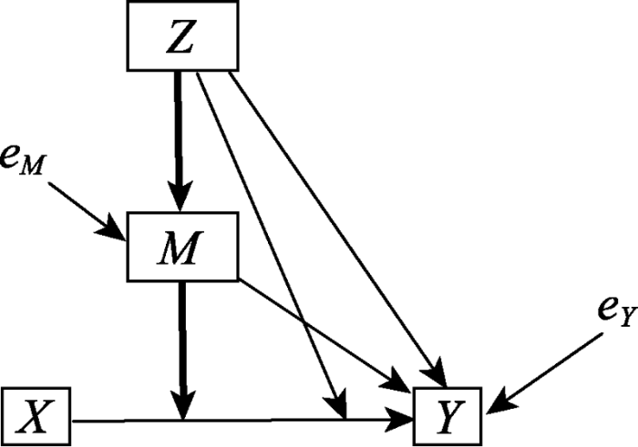
虽然meMO模型可以分为meMO-I型和meMO-II型, 但从可解释性和变量具体意义的角度, meMO-II模型更有意义, 有很多研究者认为meMO-I模型中对应的变量没有实际意义, 应用中不应被关注(Edwards & Lambert, 2007; Hayes & Preacher, 2013)。因此, 本文重点讨论更具解释性和理论意义的meMO-II模型(Kwan & Chan, 2018; Hayes, 2018), 其对应的概念模型见图1。图1中如果Z调节了$X\to Y$间的关系, 且Z在$X\to Y$上的调节效应被变量M所中介, 这时就产生了有中介的调节(粗线条标出的间接路径), 变量M称为中介的调节变量。典型地, M可能只是部分中介了Z的调节效应, 所以Z在$X\to Y$上的直接路径被保留。图1的概念模型只是各变量之间关系的理论表达, 不能直接进行分析。只有将其转换为能够反应概念模型特征的统计模型, 才能进行进一步的数据分析。
图1
本文借助于Yuan等人(2014)的思想, 采用两层建模的思路构建图1对应的统计分析模型。图1的概念模型重点关注X对Y影响程度如何受到调节变量的影响, 即对于不同的个体i, X对Y的影响程度如何随着其在调节变量上取值的不同而变化。第一层模型描述meMO分析中自变量X对因变量Y影响程度的变化; 第二层描述Z和M对X和Y之间关系的影响, 以及调节变量Z和中介的调节变量M之间的关系。值得注意的是, 对于X和Y之间关系的变异, 在考虑了模型中涉及到的调节变量Z和中介的调节变量M外, 可能还会存在没有解释的变异, 因此在模型中增加$X\to Y$影响的随机误差项。2meMO模型可表示为:
层1:
层2:
方程(2)~(4)描述了自变量X, 调节变量Z和中介的调节变量M与因变量Y之间的关系; 方程(5)描述了调节变量Z和中介的调节变量M之间的关系。其中${{\gamma }_{d0}}$和${{\gamma }_{M0}}$分别表示因变量Y和中介的调节变量M的回归截距; ${{\gamma }_{d1}},{{\gamma }_{d2}},{{\gamma }_{c0}},{{\gamma }_{c1}},{{\gamma }_{c2}}$和${{\gamma }_{M1}}$为回归系数。假设X, Z和M是均值中心化的变量, 即$E({{Z}_{i}})=E({{X}_{i}})=E({{M}_{i}})=0$。残差项${{e}_{Yi}}={{\varepsilon }_{i}}+{{u}_{di}},{{e}_{Mi}}$和${{u}_{{{c}_{i}}}}$服从正态分布, 且$E({{e}_{Yi}})=E({{e}_{Mi}})=E({{u}_{ci}})=0,$ $\text{var}({{e}_{Yi}})=\sigma _{eY}^{2},\text{var}({{e}_{Mi}})=\sigma _{eM}^{2},~\text{var}({{u}_{ci}})=\sigma _{uc}^{2}$。${{e}_{Mi}},{{e}_{Yi}}$和${{u}_{ci}}$是相互独立的。值得注意的是, 模型虽然用两层的形式表达, 但是实际数据并不是嵌套的两层数据, 在参数估计上没法区分${{\varepsilon }_{i}}$和${{u}_{di}}$, 因此将其合并为${{e}_{Yi}}$。另外, 在模型的定义中, 允许${{c}_{i}}$存在随机变异, 以此来处理误差方差随${{X}_{i}}$变化的方差非齐性问题(后面我们再详细讨论这一问题)。2meMO模型对应的两层统计模型可用图2表示。
图2
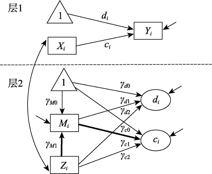
第一层模型描述meMO重点关注和解释的关系是X对Y的影响, 其中截距${{d}_{i}}$和斜率${{c}_{i}}$为随机系数; 第二层模型进一步解释Z和M对随机系数${{d}_{i}}$和${{c}_{i}}$的解释, 同时第二层模型还定义了Z和M之间的关系。具体来讲, 方程(3)描述了模型中Y对X回归的截距${{d}_{i}}$受到的影响(除了X外直接指向因变量Y的变量); 方程(4)描述了X对Y的回归系数${{c}_{i}}$受到的调节(指向X到Y回归线上的变量), 其中${{\gamma }_{c0}}$表示X对Y的主效应, ${{\gamma }_{c1}}$表示M对X和Y之间关系的调节, ${{\gamma }_{c2}}$表示Z对X和Y之间关系的直接调节; 方程(5)描述了M对Z的回归。这种采用两层定义模型的方式突出了meMO模型中解释的重点是X和Y之间的关系(层1)如何被调节(直接调节或间接调节), 从而可有效区分meMO与moME所关注问题的差异。
下面通过合并模型的表达进一步明确2meMO模型和传统meMO模型的联系和区别。将(3)和(4)代入到(2)中, 得到合并模型的表达式为:
再将等式(5)代入到等式(6)中, 得到:
需要说明的是, 相比传统的meMO模型, 方程(6)和(7)多了${{u}_{ci}}{{X}_{i}}$这一项, 此项可以有效区分模型解释的重点是有中介的调节, 而非有调节的中介(我们将在讨论部分进一步解释meMO和moME的区别)。另外, 合并后的方程(7)中隐含着$X\to XM$和$XZ\to XM$两条路径以及对两条路径系数的限定(见图2和图3), 即限定$X\to XM$的路径系数与M对X回归的截距(即$1\to M$)相等, 均为${{\gamma }_{M0}}$; 限定$XZ\to XM$的路径系数与$Z\to M$相等, 均为${{\gamma }_{M1}}$。其原因如下:从方程(7)可看出, X对Y的影响为${{\gamma }_{c0}}+{{\gamma }_{c1}}{{\gamma }_{M0}}$, 包括X对Y的直接影响${{\gamma }_{c0}}$, 以及X通过XM对Y的间接影响${{\gamma }_{c1}}{{\gamma }_{M0}}$, XM对Y的影响为${{\gamma }_{c1}}$, 则可通过限定$X\to XM$为${{\gamma }_{M0}}$, 使得$X\to $ $XM\to Y$为${{\gamma }_{c1}}{{\gamma }_{M0}}$; 同理, XZ对Y的影响${{\gamma }_{c2}}+{{\gamma }_{c1}}{{\gamma }_{M1}}$, 包括XZ对Y的直接影响${{\gamma }_{c2}}$, 以及XZ通过XM对Y的间接影响${{\gamma }_{c1}}{{\gamma }_{M1}}$, XM对Y的影响为${{\gamma }_{c1}}$, 可通过限定$XZ\to XM$为${{\gamma }_{M1}}$使得$XZ\to XM\to Y$为${{\gamma }_{c2}}+$${{\gamma }_{c1}}{{\gamma }_{M1}}$。根据方程(6)和(7), 用于2meMO分析所对应的合并统计模型如图3所示。对比图2和图3, 图2的解释更加直接。
图3
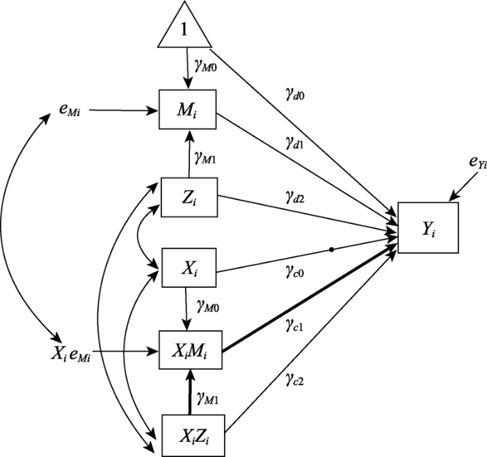
图3中X到Y路径系数上的实心圆点表对应的回归系数含有随机效应${{u}_{ci}}$, 用以描述Y的残差方差可以随X的变化而变化(方差非齐性), 传统meMO模型中不包含这项。2meMO模型允许包含随机项${{u}_{ci}}$不仅不再需要误差齐性的假设, 而且更符合实际情况。因为除了模型中考虑到的调节变量, X和Y之间的关系还有可能依赖于模型中没包含的其他调节变量, X对Y影响的随机误差项${{u}_{ci}}$也合理的刻画了这一点。除了这一随机路径, 该模型与传统的meMO对应的统计模型(Grant & Berry, 2011; Liu et al., 2012)相比, 传统模型中$XZ\to XM$和$X\to XM$的路径自由估计, 而在我们推导的统计模型中这两条路径分别限定为与Z对M回归的斜率和截距相等, 对于模型的自由度增加了2。除了随机效应${{u}_{ci}}$外, 虽然2meMO对应合并统计模型中的其他部分与Kwan和Chan (2018)从另一视角推导的meMO的统计模型相同, 但两者建构和解释meMO影响效应的思路存在本质差异。2meMO分层统计模型(图2)与概念模型的对应关系更清晰, 模型中关于X和Y之间关系变异的解释也更易于理解, 可以围绕X和Y之间关系变异(ci)的解释, 定义调节变量Z的总调节效应、直接调节效应以及间接调节效应, 而且这一定义效应量的思路同样适用于${{u}_{ci}}=0$的模型。
3 meMO效应量的定义
在方程(2)~(5)所定义的2meMO模型中, 将(5)代入(4), 可以将X对Y总的影响效应${{c}_{i}}$表示为:
第一项${{\gamma }_{c0}}+{{\gamma }_{c1}}{{\gamma }_{M0}}$表示X对Y的影响, 其中${{\gamma }_{c0}}$表示X对Y的直接影响, ${{\gamma }_{c1}}{{\gamma }_{M0}}$表示X通过XM对Y的间接影响, 这一项与调节变量Z的取值无关。第二项$({{\gamma }_{c2}}+{{\gamma }_{c1}}{{\gamma }_{M1}})$表示调节变量Z对$X\to Y$的总调节效应, 其中${{\gamma }_{c2}}$是Z对$X\to Y$的直接调节效应, ${{\gamma }_{c1}}{{\gamma }_{M1}}$是Z通过M对$X\to Y$的中介的调节效应(对应概念模型(图2)中粗体线表示的Z通过M对X和Y之间回归系数的影响, 对应于合并统计模型(图3)中的$XZ\to XM\to Y$), ${{\gamma }_{c1}}{{\gamma }_{M1}}$即为meMO模型关注的有中介的调节, 记为${{\gamma }_{meMO}}$。推断统计中将中介调节效应的检验转换为检验${{H}_{0}}:{{\gamma }_{meMO}}=0$是否显著的问题。实际中, 经常通过对调节变量Z取给定的值z (如高于或低于均值1个标准差), 计算得到${{\gamma }_{c1}}{{\gamma }_{M1}}z$, 来解释调节变量Z取不同值时, Z通过中介变量M对X和Y之间关系的影响程度(简单meMO)。类似于调节效应中简单效应差异的检验, 对于给定的不同调节效应值${{Z}_{1}}={{z}_{1}}$和${{Z}_{2}}={{z}_{2}}$, 可得到中介调节效应差异$di{{f}_{meMO}}={{\gamma }_{c1}}{{\gamma }_{M1}}({{z}_{1}}-{{z}_{2}})$, 实际中也可对${{H}_{0}}:di{{f}_{meMO}}=0$进行检验, 以回答调节变量Z取不同值${{z}_{1}}$和${{z}_{2}}$时, 中介调节作用是否存在差异。
X对Y影响程度的变异, 即${{c}_{i}}$的方差为:
下面我们基于${{c}_{i}}$变异的不同来源来定义可以测量meMO大小的效应量。第一个效应量
为调节变量Z对回归系数${{c}_{i}}$总变异所解释的比例, 可以用来测量X对Y影响的变异中, 调节变量Z所能解释的总变异所占的比例。效应量
则描述了变量Z的直接调节效应对回归系数${{c}_{i}}$总变异所解释的比例, 可以用来测量调节变量Z对$X\to Y$路径直接调节效应的大小。而效应量
描述了变量Z通过中介的调节变量M的间接调节效应(也叫做有中介的调节)对回归系数${{c}_{i}}$总变异所解释的比例, 可以用来衡量调节变量Z通过中介的调节变量M对$X\to Y$路径系数的调节效应的大小。值得注意的是, 基于变异分解所定义的效应量, 由于直接调节效应对应的路径系数${{\gamma }_{c2}}$与间接调节效应对应的路径系数${{\gamma }_{c1}}{{\gamma }_{M1}}$均与变量Z有关, 两者之间不具有独立性。因此, 通过路径系数定义的变异解释率不具有可加性, 其直接调节效应量与间接调节效应量的和并不等于总的调节效应量, 即:${{\phi }_{MO\_tot}}\ne $ ${{\phi }_{MO\_dir}}+{{\phi }_{MO\_ind}}$。
当方差齐性假设被满足时, 回归系数${{c}_{i}}$的残差随机部分为零, 即${{u}_{ci}}=0$, 等式(2)~(5)中的模型被还原为传统的有中介的调节模型(简称为meMO), 上面定义的公式(10)~(12)被简化为以下公式。
总调节效应:
直接的调节效应:
中介的调节效应:
这里, 我们使用上标(f)来区分定义中不包含的X对Y未解释的随机残差。
公式(13)~(15)同样适用于2meMO模型, 其分母表示的意义是在不考虑$X\to Y$影响系数的随机误差(${{u}_{ci}}$)时, 调节变量Z对$X\to Y$影响系数的调节。其包含可解释的调节${{({{\gamma }_{c2}}+{{\gamma }_{c1}}{{\gamma }_{M1}})}^{2}}\text{var}({{Z}_{i}})$和通过中介的调节变量M间接未解释的调节$\gamma _{c1}^{2}\sigma _{eM}^{2}$两部分。在可解释的调节中包含调节变量Z直接的调节和通过中介的调节变量M间接的调节。因此, 不论是误差方差满足齐性的条件还是误差方差依赖于X的情况, 我们都给出了测量有中介调节效应的效应量指标。公式(13)~(15)同时适用于meMO和2meMO模型, 而公式(10)~(12)仅适用于2meMO模型。
由于本研究拓展的2meMO模型随机部分参数更复杂, 极大似然估计方法会遇到基本假设(误差方差齐性)被违背的问题。考虑到贝叶斯估计在处理复杂模型, 尤其是含有更复杂的随机变异模型时更加灵活的优势(Wang Preacher, 2015; Muthén & Asparouhov, 2012; Asparouhov & Muthén, 2020), 我们使用贝叶斯方法估计2meMO中的参数及效应量。为了便于比较, 贝叶斯估计方法也用于meMO模型的参数估计。在指定模型和先验分布后, 采用马尔可夫链蒙特卡洛(Markov Chain Monte Carlo, MCMC) Gibbs采样获得模型参数的后验分布(Gilks et al., 1996)。关于Gibbs采样收敛性的检查, 使用Gelman-Rubin势能缩减(potential scale reduction, PSR)统计量。根据Brooks和Gelman (1998)的研究, 如果PSR统计量小于1.05, 则认为参数估计达到收敛。对于收敛样本, 我们将参数的贝叶斯估计定义为其后验分布的均值(称为后验均值, 实际中也可用中位数), 并且使用收敛样本的标准差获得后验标准差。基于每个参数后验分布2.5%和97.5%的分位数, 得到95%可信区间(Credibility Interval, CI)(Song & Lee, 2012)。
4 模拟研究
本研究通过模拟研究的方法, 比较不同条件下, meMO和2meMO在参数估计精度和效应量估计方面的表现。通过meMO和2meMO的比较, 验证方差齐性条件不满足时, 拓展的2meMO模型的必要性。
4.1 模拟设计
对于方程(2)~(5), 参考Wen等人(2010)以及Liu等人(2020)的模拟条件, 参数真值的设定如下:(1)调节回归系数${{\gamma }_{c1}}$的大小取3个水平:0、0.2和0.4; (2)随机误差${{u}_{ci}}$的方差$\sigma _{uc}^{2}$取3个水平:0、0.25和0.5; (3)样本量取4个水平:100、200、500和1000。注意条件$\sigma _{uc}^{2}=~$0时, 表示Y的误差方差满足齐性假设, 这时对应的真模型为meMO模型。其他条件的设定如下:将截距${{\gamma }_{M0}}$和${{\gamma }_{d0}}$设置为0; 将$X\to Y,Z\to Y,M\to Y$和$Z\to M$的主效应均设置为0.4, 即${{\gamma }_{d1}}={{\gamma }_{d2}}={{\gamma }_{c0}}={{\gamma }_{M1}}=0.4$; ${{Z}_{i}}$对$X\to Y$路径的直接调节效应设置为0.2, 即${{\gamma }_{c2}}=0.2$。自变量$X$, 调节变量$Z$, 误差项${{e}_{Mi}}$和${{e}_{Yi}}$服从标准正态分布N(0,1)。共有36个条件, 每个条件重复500次。基于2meMO模型, 使用R软件(R Core Team, 2016)模拟生成数据。根据公式(10)~(15)可以得到对应于${{\gamma }_{c1}}$和$\sigma _{uc}^{2}$组合下, 效应量的真值, 结果见表1。
表1 模拟设计条件对应的效应量真值
| ${{\gamma }_{c1}}$ | 0 | 0.2 | 0.4 | ||||||
|---|---|---|---|---|---|---|---|---|---|
| $\sigma _{uc}^{2}$ | 0 | 0.25 | 0.5 | 0 | 0.25 | 0.5 | 0 | 0.25 | 0.5 |
| $\phi _{MO\_tot}^{\left( f \right)}$ | 1 | 1 | 1 | 0.6622 | 0.6622 | 0.6622 | 0.4475 | 0.4475 | 0.4475 |
| $\phi _{MO\_dir}^{\left( f \right)}$ | 1 | 1 | 1 | 0.3378 | 0.3378 | 0.3378 | 0.1381 | 0.1381 | 0.1381 |
| $\phi _{meMO}^{\left( f \right)}$ | 0 | 0 | 0 | 0.0541 | 0.0541 | 0.0541 | 0.0884 | 0.0884 | 0.0884 |
| ${{\phi }_{MO\_tot}}$ | 1 | 0.1379 | 0.7410 | 0.6622 | 0.2128 | 0.1268 | 0.4475 | 0.2402 | 0.1641 |
| ${{\phi }_{MO\_dir}}$ | 1 | 0.1379 | 0.7410 | 0.3378 | 0.1086 | 0.0647 | 0.1381 | 0.0741 | 0.0507 |
| ${{\phi }_{meMO}}$ | 0 | 0 | 0 | 0.0541 | 0.0174 | 0.0103 | 0.0884 | 0.0474 | 0.0324 |
4.2 数据分析和评价指标
对于2meMO模型和meMO模型, 使用JAGS (Plummer, 2015)和R软件(R Core Team, 2016)中的程序包“R2jags”进行贝叶斯估计, 共迭代15000次, 采用最后5000次迭代获得参数的后验分布, 即内燃(burn in)的值设定为10000。对于模型中参数先验分布的选择, 基于文献建议(e.g., Song & Lee, 2012; Wang & Preacher, 2015), 对于回归系数$\gamma =({{\gamma }_{M0}},{{\gamma }_{M1}},{{\gamma }_{d0}},{{\gamma }_{d1}},{{\gamma }_{d2}},{{\gamma }_{c0}},{{\gamma }_{c1}},{{\gamma }_{c2}})$采用独立正态分布的先验, 对于误差方差${{\sigma }^{2}}=(\sigma _{eM}^{2},\sigma _{eY}^{2},\sigma _{uc}^{2})$采用独立的逆伽马分布的先验, 这些先验是回归分析和结构方程模型常用的半共轭先验(Gelman et al., 2004)。具体而言, 对于回归系数, 设定先验分布为:${{\gamma }_{k}}\tilde{\ }N(0,{{10}^{6}})$; 对于误差方差, 设定先验分布为:$\sigma _{l}^{2}\tilde{\ }IGamma(0.001,0.001)$。链条数设为3, 为了降低后验分布间的自相关和节约存储空间, 将抽取后验分布的间隔设定为10 (即thin=10)。感兴趣的参数包括中介调节效应${{\gamma }_{meMO}}$和中介调节效应的差异$di{{f}_{meMO}}$, 取$Z=1$来评估的简单meMO效应(${{\gamma }_{meMO}}$)的估计, 取$Z=1$和$Z=-1$来检验调节变量Z取不同值时两个简单meMO效应的差异($di{{f}_{meMO}}$)。
对于参数${{\gamma }_{meMO}}$和$di{{f}_{meMO}}$, 使用参数估计的偏差(Bias)、均方误差(MSE)、95%可信区间的覆盖率、检验力和第一类错误5个指标评估参数估计的精度。对于效应量, 采用前3个指标评估其估计精度。同时采用meMO和2meMO模型进行估计, 对于2meMO模型, 可以得到$\phi _{MO\_tot}^{(f)},\phi _{MO\_dir}^{(f)},\phi _{meMO}^{(f)},$ ${{\phi }_{MO\_tot}},{{\phi }_{MO\_dir}}$和${{\phi }_{meMO}}$的估计结果, 对于meMO模型, 可得到前3个效应量的估计值。
偏差(Bias)和均方误差(MSE)的定义如下:
其中, $\bar{\theta }=\sum _{r=1}^{R}{{\hat{\theta }}_{r}}/R$表示R=500次重复参数估计
的均值, ${{\hat{\theta }}_{r}}$为第r次重复的参数估计值。
95%可信区间的覆盖率是指R=500次重复中贝叶斯估计得到的后验分布中第2.5%和第97.5%可信区间内包含参数真值的次数所占的比例。检验力是在参数对应的真值不为0的条件下, R=500次重复中能够检验出参数显著不为零的次数所占的比例。第一类错误是在参数对应的真值为0的条件下, R=500次重复中错误的检验出参数显著不为0的次数所占的比例。
4.3 结果
对于每一组模拟条件, 模型中所有参数对应的PSR统计量均小于1.05, 说明对于meMO和2meMO模型, 贝叶斯估计均不存在不收敛的问题。
4.3.1 ${{\gamma }_{meMO}}$和$di{{f}_{meMO}}$的估计精度
表2给出了有中介调节效应估计值${{\hat{\gamma}_{meMO}}}$的偏差, 均方误差, 95%可信区间覆盖率和拒绝率。对于拒绝率, ${{\gamma }_{meMO}}=0$时拒绝率的值代表第一类错误率, ${{\gamma }_{meMO}}\ne 0$时拒绝率的值代表检验力。可以看出, 对于参数估计的偏差和均方误差两种模型得到的参数估计结果几乎没有差异(差异在小数点后第四位)。在满足方差齐性的条件下, meMO模型与2meMO模型得到的参数估计结果也基本一致。但是当方差齐性条件不满足时, 随着$\sigma _{uc}^{2}$方差增加, 对于95%可信区间覆盖率和第一类错误的结果, 2meMO模型的结果明显更有优势。对于检验力的结果, meMO在小样本时略高于2meMO, 其主要原因可能是因为这些条件下, meMO模型过高的第一类错误导致检验力的虚假提高。随着样本量和调节回归系数${{\gamma }_{{{c}_{1}}}}$的增加, 检验力提高。
表2 两种模型得到的${{\gamma }_{meMO}}$的偏差, 均方误差, 95%可信区间覆盖率和拒绝率
| 评价指标 | ${{\gamma }_{c1}}$ | $\sigma _{uc}^{2}$ | 真值 | meMO | 2meMO | ||||||
|---|---|---|---|---|---|---|---|---|---|---|---|
| 100 | 200 | 500 | 1000 | 100 | 200 | 500 | 1000 | ||||
| Bias | 0 | 0 | 0 | 0.002 | 0.001 | 0.000 | -0.001 | 0.002 | 0.001 | 0.000 | -0.001 |
| 0.25 | 0 | -0.002 | -0.001 | 0.000 | 0.001 | -0.001 | -0.001 | 0.000 | 0.001 | ||
| 0.5 | 0 | 0.003 | 0.000 | 0.001 | -0.001 | 0.003 | 0.000 | 0.001 | -0.001 | ||
| 0.2 | 0 | 0.08 | -0.002 | -0.002 | 0.000 | 0.001 | -0.002 | -0.002 | 0.000 | 0.001 | |
| 0.25 | 0.08 | -0.006 | 0.000 | 0.000 | 0.000 | -0.006 | 0.000 | 0.000 | 0.000 | ||
| 0.5 | 0.08 | -0.002 | 0.002 | -0.002 | 0.001 | -0.001 | 0.000 | -0.002 | 0.002 | ||
| 0.4 | 0 | 0.16 | 0.000 | 0.001 | 0.001 | 0.000 | 0.000 | 0.001 | 0.001 | 0.000 | |
| 0.25 | 0.16 | -0.004 | -0.001 | 0.002 | 0.000 | -0.004 | -0.001 | 0.002 | 0.000 | ||
| 0.5 | 0.16 | -0.002 | -0.004 | 0.000 | 0.002 | -0.002 | -0.003 | 0.001 | 0.002 | ||
| MSE | 0 | 0 | 0 | 0.002 | 0.001 | 0.000 | 0.000 | 0.002 | 0.001 | 0.000 | 0.000 |
| 0.25 | 0 | 0.003 | 0.001 | 0.001 | 0.000 | 0.003 | 0.001 | 0.001 | 0.000 | ||
| 0.5 | 0 | 0.004 | 0.002 | 0.001 | 0.000 | 0.004 | 0.002 | 0.001 | 0.000 | ||
| 0.2 | 0 | 0.08 | 0.002 | 0.001 | 0.000 | 0.000 | 0.002 | 0.001 | 0.000 | 0.000 | |
| 0.25 | 0.08 | 0.004 | 0.002 | 0.001 | 0.000 | 0.003 | 0.002 | 0.001 | 0.000 | ||
| 0.5 | 0.08 | 0.005 | 0.002 | 0.001 | 0.001 | 0.005 | 0.002 | 0.001 | 0.000 | ||
| 0.4 | 0 | 0.16 | 0.004 | 0.002 | 0.001 | 0.000 | 0.004 | 0.002 | 0.001 | 0.000 | |
| 0.25 | 0.16 | 0.005 | 0.002 | 0.001 | 0.000 | 0.005 | 0.002 | 0.001 | 0.000 | ||
| 0.5 | 0.16 | 0.006 | 0.003 | 0.001 | 0.001 | 0.005 | 0.003 | 0.001 | 0.001 | ||
| 覆盖率 | 0 | 0 | 0 | 0.952 | 0.942 | 0.942 | 0.942 | 0.952 | 0.956 | 0.944 | 0.940 |
| 0.25 | 0 | 0.908 | 0.920 | 0.918 | 0.872 | 0.940 | 0.956 | 0.942 | 0.932 | ||
| 0.5 | 0 | 0.912 | 0.874 | 0.852 | 0.870 | 0.948 | 0.952 | 0.936 | 0.948 | ||
| 0.2 | 0 | 0.08 | 0.962 | 0.950 | 0.966 | 0.924 | 0.968 | 0.954 | 0.972 | 0.926 | |
| 0.25 | 0.08 | 0.920 | 0.918 | 0.922 | 0.908 | 0.930 | 0.944 | 0.956 | 0.946 | ||
| 0.5 | 0.08 | 0.894 | 0.882 | 0.884 | 0.882 | 0.928 | 0.946 | 0.936 | 0.944 | ||
| 0.4 | 0 | 0.16 | 0.960 | 0.948 | 0.958 | 0.950 | 0.962 | 0.950 | 0.958 | 0.946 | |
| 0.25 | 0.16 | 0.935 | 0.937 | 0.930 | 0.933 | 0.960 | 0.948 | 0.942 | 0.962 | ||
| 0.5 | 0.16 | 0.926 | 0.928 | 0.896 | 0.882 | 0.946 | 0.954 | 0.940 | 0.940 | ||
| 拒绝率 | 0 | 0 | 0 | 0.048 | 0.058 | 0.058 | 0.058 | 0.048 | 0.044 | 0.056 | 0.060 |
| 0.25 | 0 | 0.092 | 0.080 | 0.082 | 0.129 | 0.060 | 0.044 | 0.058 | 0.068 | ||
| 0.5 | 0 | 0.088 | 0.126 | 0.148 | 0.130 | 0.052 | 0.048 | 0.064 | 0.052 | ||
| 0.2 | 0 | 0.08 | 0.438 | 0.762 | 0.998 | 1.000 | 0.399 | 0.760 | 0.996 | 1.000 | |
| 0.25 | 0.08 | 0.390 | 0.650 | 0.970 | 1.000 | 0.314 | 0.606 | 0.950 | 1.000 | ||
| 0.5 | 0.08 | 0.362 | 0.600 | 0.882 | 0.994 | 0.269 | 0.488 | 0.838 | 0.990 | ||
| 0.4 | 0 | 0.16 | 0.938 | 1.000 | 1.000 | 1.000 | 0.926 | 1.000 | 1.000 | 1.000 | |
| 0.25 | 0.16 | 0.834 | 0.996 | 1.000 | 1.000 | 0.808 | 0.952 | 1.000 | 1.000 | ||
| 0.5 | 0.16 | 0.794 | 0.970 | 1.000 | 1.000 | 0.730 | 0.964 | 1.000 | 1.000 | ||
注:覆盖率低于0.9, 第一类错误率高于8%的值用粗体字表示。${{\gamma }_{meMO}}=0$时拒绝率的值代表第一类错误率, ${{\gamma }_{meMO}}\ne 0$时拒绝率的值代表检验力。
$di{{f}_{meMO}}$与${{\gamma }_{\text{meMO}}}$所得结论一致。传统meMO和2meMO模型的偏差都很小。在方差齐性的条件下, 两种模型中Bias、MSE、对应的95%可信区间的覆盖率和第一类错误的差异很小。然而, 在误差方差非齐性条件下, 2meMO对$\text{ }\!\!~\!\!\text{ }di{{f}_{meMO}}$进行估计更加准确, 同时2meMO对应的95%可信区间的覆盖率更接近95%。2meMO方法在控制第一类错误率方面表现更好, 随着$\sigma _{uc}^{2}$值的增加, meMO的第一类错误率有所增大。
4.3.2 效应量的估计结果
对于总体中存在中介调节效应(${{\gamma }_{c1}}=0.20.4$)时, 可以使用meMO模型和2meMO模型, 利用公式(13)~(15)得到效应量$\phi _{MO\_tot}^{\left( f \right)},\phi _{MO\_dir}^{\left( f \right)}$和$\phi _{meMO}^{\left( f \right)}$的估计值; 当回归系数${{c}_{i}}$对应的误差方差$\sigma _{uc}^{2}\ne 0$时, 可以采用2meMO模型, 利用公式(10)~(12)得到效应量${{\phi }_{MO\_tot}},{{\phi }_{MO\_dir}}$和${{\phi }_{meMO}}$的估计值。效应量的结果表明, 不同测量指标的结果表现出相同的模式, 所以文中仅给出$\phi _{meMO}^{\left( f \right)}$和${{\phi }_{meMO}}$的结果。
表3给出了两种模型得到的$\phi _{meMO}^{\left( f \right)}$的估计值。样本量越大, $\sigma _{uc}^{2}$的值越小, $\phi _{meMO}^{\left( f \right)}$的估计精度越高。在$\sigma _{uc}^{2}=0$的情况下, meMO模型和2meMO模型间的差异很小。但是, 当$\sigma _{uc}^{2}\ne 0$时, 2meMO的结果更加精确, 并且随着$\sigma _{uc}^{2}$值的增加, 2meMO模型相对于meMO模型的优势变得越来越明显。
表3 两种模型得到的效应量$\phi _{meMO}^{(f)}$估计的偏差, 均方误差, 95%可信区间覆盖率
| 评价指标 | ${{\gamma }_{c1}}$ | $\sigma _{uc}^{2}$ | 真值 | moME | 2moME | ||||||
|---|---|---|---|---|---|---|---|---|---|---|---|
| 100 | 200 | 500 | 1000 | 100 | 200 | 500 | 1000 | ||||
| Bias | 0.2 | 0 | 0.054 | 0.014 | 0.006 | 0.002 | 0.002 | 0.015 | 0.006 | 0.003 | 0.002 |
| 0.25 | 0.054 | 0.015 | 0.009 | 0.004 | 0.001 | 0.016 | 0.010 | 0.004 | 0.001 | ||
| 0.5 | 0.054 | 0.023 | 0.013 | 0.003 | 0.003 | 0.022 | 0.012 | 0.003 | 0.003 | ||
| 0.4 | 0 | 0.088 | 0.003 | 0.001 | 0.001 | 0.001 | 0.004 | 0.001 | 0.001 | 0.001 | |
| 0.25 | 0.088 | 0.000 | 0.001 | 0.002 | -0.001 | 0.000 | 0.001 | 0.002 | -0.001 | ||
| 0.5 | 0.088 | 0.001 | -0.002 | 0.002 | 0.001 | 0.002 | -0.002 | 0.001 | 0.001 | ||
| MSE | 0.2 | 0 | 0.054 | 0.003 | 0.001 | 0.001 | 0.000 | 0.003 | 0.001 | 0.001 | 0.000 |
| 0.25 | 0.054 | 0.003 | 0.002 | 0.001 | 0.000 | 0.003 | 0.002 | 0.001 | 0.000 | ||
| 0.5 | 0.054 | 0.004 | 0.002 | 0.001 | 0.001 | 0.003 | 0.002 | 0.001 | 0.000 | ||
| 0.4 | 0 | 0.088 | 0.002 | 0.001 | 0.000 | 0.000 | 0.002 | 0.001 | 0.000 | 0.000 | |
| 0.25 | 0.088 | 0.003 | 0.001 | 0.001 | 0.000 | 0.003 | 0.001 | 0.001 | 0.000 | ||
| 0.5 | 0.088 | 0.003 | 0.002 | 0.001 | 0.000 | 0.003 | 0.001 | 0.001 | 0.000 | ||
| 覆盖率 | 0.2 | 0 | 0.054 | 0.962 | 0.940 | 0.956 | 0.926 | 0.958 | 0.944 | 0.954 | 0.922 |
| 0.25 | 0.054 | 0.958 | 0.926 | 0.922 | 0.914 | 0.970 | 0.950 | 0.962 | 0.948 | ||
| 0.5 | 0.054 | 0.958 | 0.902 | 0.882 | 0.874 | 0.980 | 0.954 | 0.952 | 0.934 | ||
| 0.4 | 0 | 0.088 | 0.968 | 0.952 | 0.948 | 0.954 | 0.966 | 0.952 | 0.948 | 0.950 | |
| 0.25 | 0.088 | 0.964 | 0.944 | 0.948 | 0.952 | 0.964 | 0.944 | 0.948 | 0.952 | ||
| 0.5 | 0.088 | 0.932 | 0.908 | 0.914 | 0.874 | 0.950 | 0.940 | 0.956 | 0.932 | ||
注:覆盖率低于0.9的值用粗体字表示。
表4给出了2meMO模型得到的效应量${{\phi }_{meMO}}$的估计值。从结果可以看出, 在所有条件下, MSE值都很小, ${{\phi }_{meMO}}$对应的95%可信区间的覆盖率也接近95%。随着$\sigma _{uc}^{2}$和样本量的增加, ${{\phi }_{meMO}}$估计的精度越来越高。但是, 值得注意的是, 当样本量较小时, ${{\phi }_{meMO}}$估计的偏差较大, 尤其是对于较小的有中介的调节效应而言。因此, 在实践中, 为了获得对${{\phi }_{meMO}}$更准确的估计, 可能需要更大的样本量, 或者类似于传统回归分析中对R2的估计, 需要对其偏度进行校正。
表4 2meMO模型得到的效应量${{\phi }_{meMO}}$估计的偏差, 均方误差, 95%可信区间覆盖率
| 评价指标 | ${{\gamma }_{c1}}$ | $\sigma _{uc}^{2}$ | 真值 | 100 | 200 | 500 | 1000 |
|---|---|---|---|---|---|---|---|
| Bias | 0 | 0 | 0 | 0.040 | 0.024 | 0.013 | 0.007 |
| 0.25 | 0 | 0.030 | 0.016 | 0.005 | 0.002 | ||
| 0.5 | 0 | 0.023 | 0.009 | 0.003 | 0.001 | ||
| 0.2 | 0 | 0.0541 | -0.002 | -0.005 | -0.006 | -0.004 | |
| 0.25 | 0.0174 | 0.021 | 0.016 | 0.006 | 0.002 | ||
| 0.5 | 0.0104 | 0.020 | 0.010 | 0.002 | 0.002 | ||
| 0.4 | 0 | 0.0884 | -0.009 | -0.008 | -0.005 | -0.004 | |
| 0.25 | 0.0474 | 0.013 | 0.011 | 0.006 | 0.002 | ||
| 0.5 | 0.0324 | 0.017 | 0.007 | 0.003 | 0.002 | ||
| MSE | 0 | 0 | 0 | 0.003 | 0.001 | 0.000 | 0.000 |
| 0.25 | 0 | 0.002 | 0.001 | 0.000 | 0.000 | ||
| 0.5 | 0 | 0.001 | 0.000 | 0.000 | 0.000 | ||
| 0.2 | 0 | 0.0541 | 0.002 | 0.001 | 0.000 | 0.000 | |
| 0.25 | 0.0174 | 0.001 | 0.001 | 0.000 | 0.000 | ||
| 0.5 | 0.0104 | 0.001 | 0.001 | 0.000 | 0.000 | ||
| 0.4 | 0 | 0.0884 | 0.002 | 0.001 | 0.000 | 0.000 | |
| 0.25 | 0.0474 | 0.002 | 0.001 | 0.000 | 0.000 | ||
| 0.5 | 0.0324 | 0.002 | 0.001 | 0.000 | 0.000 | ||
| 覆盖率 | 0.2 | 0 | 0.0541 | 0.932 | 0.936 | 0.948 | 0.922 |
| 0.25 | 0.0174 | 0.978 | 0.954 | 0.954 | 0.936 | ||
| 0.5 | 0.0104 | 0.976 | 0.964 | 0.940 | 0.948 | ||
| 0.4 | 0 | 0.0884 | 0.946 | 0.946 | 0.950 | 0.932 | |
| 0.25 | 0.0474 | 0.962 | 0.946 | 0.936 | 0.936 | ||
| 0.5 | 0.0324 | 0.960 | 0.962 | 0.932 | 0.948 |
注:对于2meMO模型, 由于方差估计大于0, 置信区间的覆盖率均不包含0。
5 应用案例
5.1 数据和模型
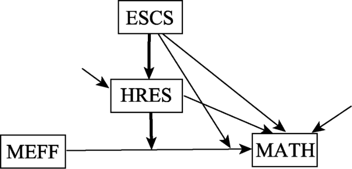
为了便于2meMO模型与meMO模型的比较, 这里我们采用Kwan和Chan (2018)研究中所用的数据(下载地址:http://dx.doi.org/10.1037/met0000160. supp)。其数据来源于2012年OECD (Organization for Economic Cooperation and Development)组织的PISA测试(the Program for International Student Assessment, PISA), 具体介绍见Kwan和Chan (2018)研究中的介绍。该数据样本量为3047, 分析的变量包括:因变量数学学业成绩(MATH), 自变量数学自我效能(MEFF), 调节变量社会经济地位(ESCS)以及中介的调节变量家庭教育资源(HRES)。模型假设:ESCS可以调节MEFF与MATH之间的关系, ESCS较低的学生, MEFF对MATH的影响较强, 而ESCS较高的学生, MEFF对MATH的影响较弱; 进一步, ESCS对MEFF与MATH之间关系的调节作用被HRES所中介, ESCS高的学生拥有较多的HRES, 所以MEFF对MATH的影响较弱。对应的概念模型见图4, 分析的模型包括传统meMO模型和2meMO模型, 分析过程中对MEFF、ESCS和HRES做均值中心化处理。为了帮助应用者理解和便于应用者使用分析程序, 我们在网络版附录中给出了默认先验设置时Mplus 8.3的语句。需要再次强调的是这里的数据是单层次结构, 在Mplus中我们借助于多层模型采用贝叶斯估计方法实现2meMO的参数估计, 一个个体就是一个cluster。
图4
5.2 分析结果
对于meMO模型和2meMO模型, 在默认先验设置条件下模型中所有参数对应的PSR统计量均介于1.00到1.02之间, 进一步检查3条不同链的轨迹图发现不同链条收敛到同样的后验分布。表6给出了两个模型的参数估计结果、中介的调节效应估计值和本研究提出的效应量指标。2meMO模型对应的DIC (Deviance Information Criteria)为78000.4, meMO模型对应的DIC为78069.2, 两个模型对应的DIC的差异ΔDIC = 68.8, 2meMO模型的DIC较小, 根据Cain和Zhang (2019)所建议的ΔDIC > 7的模型比较标准, 2meMO模型的拟合优于meMO模型。
从表5的结果可以看出, 两个模型得到的参数估计结果在大多数参数上相差不大。meMO和2meMO估计得到的有中介调节效应的后验均值分别为-2.019和-2.165, 对应的95% CI分别为(-3.439, -0.614)和(-3.757, -0.673), CI不包含0, 说明有中介的调节效应显著。2meMO模型结果表明, 第一层数学自我效能对数学成绩影响的总变异的后验均值$~\widehat{\text{var}}\left( {{c}_{i}} \right)=484.239$, 95%的CI为(229.158, 737.546); 数学自我效能对数学成绩影响的变异中可以被调节变量社会经济地位和中介的调节变量家庭教育资源联合解释部分${{({{\gamma }_{c2}}+{{\gamma }_{c1}}{{\gamma }_{M1}})}^{2}}\text{var}({{Z}_{i}})+$ $\gamma _{c1}^{2}\sigma _{eM}^{2}$的后验均值为46.643, 95%的CI为(13.412, 83.211)。由贝叶斯估计得到的效应量${{\hat{\phi }}_{MO\_tot}},$ ${{\hat{\phi }}_{MO\_dir}}$和${{\hat{\phi }}_{meMO}}$的后验均值分别为0.059,0.025和0.010, 95% CI分别为(0.007, 0.122), (0.000, 0.068)和(0.000, 0.023), 说明在数学成绩对数学自我效能影响的总变异中, 社会经济地位调节效应的总解释率的后验均值为5.9%, 社会经济地位直接调节效应的解释率的后验均值为2.5%, 间接调节效应(即有中介的调节效应)的解释率的后验均值为1.0%。分母上去掉误差${{u}_{ci}}$的方差后, 得到效应量$\hat{\phi }_{MO\_tot}^{\left( f \right)},\hat{\phi }_{MO\_dir}^{\left( f \right)}$和$\hat{\phi }_{meMO}^{\left( f \right)}$的后验均值的估计值分别为0.637, 0.275和0.106, 95% CI分别为(0.296, 1.000), (0.000,0.667)和(0.000,0.206), 说明在不考虑数学自我效能→数学学业成绩影响系数的随机误差(${{u}_{ci}}$)时, 在社会经济地位和家庭教育资源联合解释的数学自我效能对数学成绩影响的变异中, 社会经济地位总解释率的后验均值为63.7%, 社会经济地位直接调节效应的解释率的后验均值为27.5%, 间接调节效应的解释率的后验均值为10.6%。本例中, ${{\hat{\phi }}_{meMO}}$与$\hat{\phi }_{meMO}^{\left( f \right)}$在数值上差异较大, 其主要原因是因为所用分母的差异, 也从另一角度说明了2meMO模型中考虑$X\to Y$随机误差的意义。
表5 meMO和2meMO模型参数估计结果
| 统计量 | meMO | 2meMO | ||
|---|---|---|---|---|
| 后验均值 | 后验标准差 | 后验均值 | 后验标准差 | |
| 路径系数 | ||||
| ESCS→HRES (${{\hat{\gamma }}_{M1}}$) | 0.484*** | 0.011 | 0.484*** | 0.011 |
| MEFF→MATH (${{\hat{\gamma }}_{c0}})$ | 46.438*** | 1.385 | 48.436*** | 1.571 |
| ESCS→MATH (${{\hat{\gamma }}_{d2}})$ | 14.621*** | 1.687 | 14.368*** | 1.676 |
| HRES→MATH (${{\hat{\gamma }}_{d1}})$ | 3.492* | 1.672 | 3.418* | 1.644 |
| ESCS×MEFF→MATH (${{\hat{\gamma }}_{c2}})$ | -2.911* | 1.501 | -3.284* | 1.640 |
| HRES×MEFF→MATH (${{\hat{\gamma }}_{c1}})$ | -4.171** | 1.478 | -4.471** | 1.631 |
| ESCS×MEFF→HRES×MEFF (${{\hat{\gamma }}_{M1}})$ | 0.484*** | 0.011 | 0.484*** | 0.011 |
| 残差方差 | ||||
| $\sigma _{eM}^{2}$ | 6197.923 | 160.921 | 5668.715 | 189.195 |
| $\sigma _{eY}^{2}$ | 0.749 | 0.019 | 0.749 | 0.019 |
| $\sigma _{uc}^{2}$ | - | - | 484.239 | 130.388 |
| 有中介调节meMO | ||||
| ${{\hat{\gamma }}_{M1}}{{\hat{\gamma }}_{c1}}$ | -2.019 | 0.718 | -2.165 | 0.791 |
| 效应量 | ||||
| ${{\hat{\phi }}_{MO\_tot}}$ | - | - | 0.059 | 0.032 |
| ${{\hat{\phi }}_{MO\_dir}}$ | - | - | 0.025 | 0.022 |
| ${{\hat{\phi }}_{meMO}}$ | - | - | 0.010 | 0.007 |
| $\hat{\phi }_{MO\_tot}^{\left( f \right)}$ | 0.623 | 0.193 | 0.637 | 0.192 |
| $\hat{\phi }_{MO\_dir}^{\left( f \right)}$ | 0.261 | 0.203 | 0.275 | 0.206 |
| $\hat{\phi }_{meMO}^{\left( f \right)}$ | 0.110 | 0.057 | 0.106 | 0.056 |
本例中, 通过模型拟合的比较我们倾向于采用2meMO, 研究者可以基于感兴趣的研究问题, 在公式(10)~(15)所定义的6种不同的效应量中选择合适的效应量, 解释调节变量对$X\to Y$之间关系变异的解释。但如果实际中, 我们倾向于选择meMO模型, 则根据感兴趣的研究问题, 在公式(13)~(15)中选择合适的效应量。另外, 虽然从概念模型到统计模型的转换过程中, 我们强调模型中隐含了的对$X\to XM$和$XZ\to XM$两条路径系数的限定, 但在实际中, 这两个限定条件对于参数估计结果的影响很小, 甚至可以忽略。因此, 为了简化操作, 正如Kwan和Chan (2018)指出的实际中也可以忽略这两个限定。
6 讨论与建议
本文基于单层的数据拓展了meMO模型, 采用两层模型的框架定义了可处理误差方差非齐性的2meMO模型, 基于此模型将X对Y影响系数变异的来源进行分解, 并由此定义了可以测量总调节效应、直接调节效应和有中介的调节效应大小的效应量指标。进一步将贝叶斯方法用于2meMO模型的参数估计, 并通过Monte Carlo模拟研究考查了参数估计的精度, 并与传统的meMO模型进行了比较, 验证了2meMO模型在处理方差非齐性条件下的优势。
根据模拟研究的结果, 在方差满足齐性的假设时, meMO和2meMO得到的结果几乎没有差异, 也就是说即便在传统meMO的假设下, 2meMO也能得到无偏的精度较高的估计结果。但是在方差齐性的条件不满足时, 2meMO得到的参数估计结果在95%可信区间覆盖率和控制第一类错误上的表现优于meMO模型, 这一结果与方差非齐性的潜变量交互作用模型(Liu et al., 2020)和观测变量的调节效应回归分析模型得到的结果一致(Yang & Yuan, 2016)。2meMO模型的拓展为调节效应模型中常见的方差齐性假设条件的违背(Aguinis & Pierce, 1998; Alexander & DeShon, 1994)提供了解决思路。基于贝叶斯估计方法的可实现性以及模拟研究的结果, 我们推荐研究者使用2meMO模型处理方差非齐性的情况, 在研究中报告与感兴趣的研究问题相对应的效应量指标。
在有中介的调节效应的分析中, 本文提出的2meMO模型和对应的效应量指标有以下几方面的优点:(1)采用两层模型定义meMO统计模型的方式, 在概念模型的理解和效应量的定义上为如何区分变量的角色提供了更为一般化的框架。可以将模型关注的自变量和因变量关系的变化, 定义为层1的模型, 然后根据调节变量的定义, 在层2模型中解释调节变量对因变量和自变量之间关系的影响, 以及调节变量和中介的调节变量之间的关系。这样分层次的模型表达, 合理且有效地区分了自变量、因变量、调节变量和中介的调节变量的不同角色。(2)文中提出的效应量指标是基于自变量和因变量之间总变异(即var(ci))的分解所得到的, 这就为紧密围绕“X与Y之间关系的调节”这一关键问题, 定义合适的效应量提供了基础, 基于此所定义的效应量是围绕meMO分析所感兴趣的问题提出的, 更具可解释性, 同时也更符合效应量概念的核心内涵(e.g., Kelley & Preacher, 2012)。(3)基于2meMO提出的效应量指标, 不仅适用于方差齐性而且适用于方差非齐性的条件, 有更广的适用范围。研究者在使用过程中不用担心由于实际数据不满足方差齐性而带来的估计偏差, 检验力降低等问题。(4)2meMO模型的参数估计很容易在Gibbs取样的框架下, 借用已有的免费贝叶斯估计程序实现。如2meMO的参数估计很容易通过常用的JAGS (Plummer, 2015)、WinBugs (Lunn et al., 2012)和Mplus等软件实现。(5)更重要的是, 本文所提出的有中介的调节模型的效应量指标可满足应用研究者报告效应量的需求, 弥补了目前尚没有合适的测量meMO影响的效应量指标的局限。
另外, 本研究定义模型的方法和效应量的思路具有拓展性。本文提出的定义2meMO模型的思路, 可以在概念上为如何有效区分meMO和moME两类模型提供一些借鉴。从概念模型来看, 2meMO模型和moME-II强调的重点不同, 两者并不等价, 2meMO模型是为了解释调节效应是如何通过中介的调节变量发挥作用的; 而moME-II是为了解释中介效应是如何依赖于调节变量取值的。然而, 传统的方差齐性假设下由于两者对应的统计模型相同, 在结果解释上很难有效帮助应用研究者区分两类模型的本质区别。在两层建模的框架下, 对于moME模型可以借鉴本文的建模思路, 在层1定义与中介效应有关的路径(a和b), 而在层2解释中介路径中某个阶段的效应被调节。例如, 含有第二阶段被调节的中介模型可以定义为:
层1:
${{M}_{i}}={{a}_{i}}{{X}_{i}}+{{e}_{Mi}}$
${{Y}_{i}}={{d}_{i}}+{{b}_{i}}{{M}_{i}}+{{c}_{i}}{{X}_{i}}+{{\varepsilon }_{i}}$
层2:
${{a}_{i}}={{\gamma }_{a0}}$
${{d}_{i}}={{\gamma }_{d0}}+{{\gamma }_{d1}}{{Z}_{i}}+{{u}_{di}}$
${{b}_{i}}={{\gamma }_{b0}}+{{\gamma }_{b1}}{{Z}_{i}}+{{u}_{bi}}$
${{c}_{i}}={{\gamma }_{c0}}$
上述模型合并后的表达式中包含${{M}_{i}}{{u}_{bi}}$这一项, 而2meMO模型中包含的是${{X}_{i}}{{u}_{ci}}$, 这样统计模型的定义上可将两者加以区分。即便上述模型中不包含随机误差项${{u}_{bi}}$, 这一两层模型建构的思路也有利于研究者区分两类模型解释上的区别。未来研究中可以借鉴本文定义效应量的思路, 基于被调节的中介所关注的问题发展合适的效应量指标, 以解决有中介的调节模型与第二阶段被调节的中介模型经常出现的结果解释上被混淆的问题。
Lachowicz等人(2018)讨论了合理的效应量指标应该满足的特性(Kelley & Preacher, 2012; Preacher & Kelley, 2011; Wen & Fan, 2015)。本研究所定义的效应量指标具有以下特性。(1)效应量的定义与meMO的概念模型匹配, 在变异分解的框架下, 效应量具有可解释的尺度, 可以回答有中介调节对总调节变异方差的贡献率。(2)效应量指标不依赖于样本量, 且基于贝叶斯估计的后验分布可得到效应量的可信区间(CI)。(3)$\phi _{MO\_tot}^{\left( f \right)}$和${{\phi }_{MO\_tot}}$的取值介于0和1之间。大多数情况下, $\phi _{MO\_dir}^{\left( f \right)},\phi _{meMO}^{\left( f \right)},$ ${{\phi }_{MO\_dir}}$和${{\phi }_{meMO}}$的取值也介于0和1之间; 但在实际应用中, 可能会出现这四个效应量的数值大于1 (Lutz, 1983; Maassen & Bakker, 2001; Tzelgov & Henik, 1991), 此时说明Z对X→Y的直接调节(${{\gamma }_{c2}}$)和通过M对X→Y的间接调节(${{\gamma }_{c1}}{{\gamma }_{M1}}$)方向相反, 出现了变量之间的抑制效应(suppression effect)。
虽然所提出来的效应量具有很多优点, 但在应用时也应关注其局限性。首先, 类似于方差分析中的偏η2, var(ci)是定义效应量的基础(分母), 即效应量的解释都是以var(ci)作为比较基准的, 因此这些效应量本质上是一个相对的效应量指标。因此, 在实际应用中, 在报告效应量的时候应同时报告分母的大小, 以避免过度夸大meMO效应, 同时也有助于了解在X对Y的影响中, var(ci)的大小是否有实际的意义。研究者应该在关注var(ci)本身大小的前提下, 进一步解释meMO效应的大小。另外, 我们建议在报告效应量的时候, 同时报告本研究提出的多个效应量指标, 为全面了解变量的影响关系和强度提供更多的补充信息。同时, 应该注意基于变异分解所定义的直接调节效应和间接调解效应的效应量指标不具有可加性。
大量的研究证明不同先验分布会影响参数估计的精度(Yuan & MacKinnon, 2009), 因此, 实际中如何选择合适的先验分布是研究者应该注意的问题。本研究选取了最常用也是研究者广泛推荐的无信息先验(Browne & Draper, 2006), 结果证明即使是无信息的先验也能够得到准确的参数估计结果, 但是这一结论在实际应用中并不一定具有普适性。已有研究表明合适的有信息先验可以使得参数估计精度更高, Zondervan-Zwijnenburg等人(2017)提供了如何收集先验信息的指导。如果研究者可以得到合适的有信息的先验, 我们也鼓励采用有信息的先验以提高参数估计的精度。然而, 为了避免由于特定先验设置带来的主观性, 应当考虑采用敏感性分析进一步确认贝叶斯估计结果并不严重依赖于某个特定的先验分布(van de Schoot et al., 2017; Zondervan-Zwijnenburg et al., 2017)。
本研究只考虑了含有一个调节变量Z和一个中介的调节变量M的情况, 对于方差非齐性也只考虑了结果变量Y的方差非齐性, 未来研究中可以考虑更为复杂的meMO模型和更复杂的方差非齐性的情况。另外, 对于本研究提出的效应量指标, 如何结合效应量的特点, 给出效应量“小”、“中”、“大”的判断标准, 也是未来值得进一步研究的问题。最后, 模型中被忽略的变量、变量的测量误差和其他影响回归系数估计精度的因素也会对效应量的估计精度产生影响, 未来研究需要对这些影响因素进行更为系统和深入的探讨。
附录:meMO和2meMO模型贝叶斯估计的Mplus语句
1 meMO模型
TITLE: mediated moderation model
DATA: FILE = memo.csv;
VARIABLE: NAMES ARE ID MATH ESCS HRES MEFF CESCS CHRES CMEFF XCESCS XCHRES;
! CESCS CHRES CMEFF为均值中心化的变量;
!XCESCS= CMEFF*CESCS, XCHRES= CMEFF* CHRES;
USEVARIABLES = MATH CESCS CHRES CMEFF XCESCS XCHRES;
ANALYSIS: ESTIMATOR IS BAYES; POINT =MEAN; CHAINS =3; PROCESSORS =3;
THIN = 10; BITERATIONS=(10000); BCONVERGENCE = 0.025;
MODEL:
MATH ON CMEFF (rc0);
MATH ON CHRES (rdy1);
MATH ON CESCS (rdy2);
CHRES ON CESCS (rm1);
MATH ON XCHRES (rc1);
MATH ON XCESCS (rc2);
XCHRES ON CMEFF (rm0);
XCHRES ON XCESCS (rm1);
[CHRES MATH] (rm0 ry0);
CHRES MATH (sig_em, sig_ey);
CMEFF WITH CESCS;
CMEFF WITH XCESCS;
CESCS WITH XCESCS;
MODEL CONSTRAINT:
NEW(var_z v1 v2 v3 v5 phi_f1 phi_f2 phi_f3 );
var_z =0.935; ! z的方差;
v1 = (rc2+rc1*rm1)*(rc2+rc1*rm1)*var_z;
v2 = rc2*rc2*var_z;
v3 = rc1*rm1*rc1*rm1*var_z;
v5 = v1+rc1*rc1*sig_em;
phi_f1 = v1/v5;
phi_f2 = v2/v5;
phi_f3 = v3/v5;
MODEL CONSTRAINT:
NEW(memo memo1 memo2 dif);
memo = rc1*rm1;
memo1 = rc1*rm1*0.967; !z的标准差为0.967;
memo2 = rc1*rm1*(-0.967);
dif = memo1-memo2;
PLOT: TYPE = PLOT2;
OUTPUT: CINTERVAL(hpd) TECH8;
2 2meMO模型的Mplus语句
TITLE: two-level mediated moderation model with single-level data (2moME)
DATA: FILE = memo.csv;
VARIABLE: NAMES ARE ID MATH ESCS HRES MEFF CESCS CHRES CMEFF XCESCS XCHRES;
USEVARIABLES = MATH CESCS CHRES CMEFF XCESCS XCHRES;
CLUSTER = ID; !对于单层数据每一个组只有一名被试
WITHIN = MATH CESCS CHRES CMEFF XCESCS XCHRES; !单层数据中指定所有变量为组内变量
ANALYSIS: TYPE IS TWOLEVEL RANDOM;
ESTIMATOR IS BAYES;
POINT =MEAN;
CHAINS =3;
PROCESSORS =3;
THIN = 10;
BITERATIONS=(10000);
BCONVERGENCE = 0.025;
MODEL:
%WITHIN%
c | MATH ON CMEFF;
MATH ON CHRES (rdy1);
MATH ON CESCS (rdy2);
CHRES ON CESCS (rm1);
MATH ON XCHRES (rc1);
MATH ON XCESCS (rc2);
XCHRES ON CMEFF (rm0);
XCHRES ON XCESCS (rm1);
[CHRES] (rm0);
[MATH] (ry0);
CHRES (sig_em);
MATH;
CMEFF WITH CESCS;
CMEFF WITH XCESCS;
CESCS WITH XCESCS;
%BETWEEN%
[c] (rc0);
c (sig2_uc);
MODEL CONSTRAINT:
NEW(var_z v1 v2 v3 v4 v5 phi_1 phi_2 phi_3 phi_f1 phi_f2 phi_f3 );
var_z =0.935; ! the variance of z;
v1 = (rc2+rc1*rm1)*(rc2+rc1*rm1)*var_z;
v2 = rc2*rc2*var_z;
v3 = rc1*rm1*rc1*rm1*var_z;
v4 = v1+rc1*rc1*sig_em+sig2_uc;
v5 = v1+rc1*rc1*sig_em;
phi_1 = v1/v4;
phi_2 = v2/v4;
phi_3 = v3/v4;
phi_f1 = v1/v5;
phi_f2 = v2/v5;
phi_f3 = v3/v5;
MODEL CONSTRAINT:
NEW(memo memo1 memo2 dif);
memo = rc1*rm1;
memo1 = rc1*rm1*0.967;
memo2 = rc1*rm1*(-0.967);
dif = memo1-memo2;
PLOT: TYPE = PLOT2;
OUTPUT:
CINTERVAL(hpd);
TECH8;
参考文献
Heterogeneity of error variance and the assessment of moderating effects of categorical variables: A conceptual review
Multiple regression: Testing and interpreting interactions. London, UK:
Effect of error variance heterogeneity on the power of tests for regression slope differences
Standards for reporting on empirical social science research in AERA publications
Bayesian estimation of single and multilevel models with latent variable interactions
The moderator- mediator variable distinction in social psychological research: Conceptual, strategic, and statistical considerations
General methods for monitoring convergence of iterative simulations
A comparison of Bayesian and likelihood-based methods for fitting multilevel models
Fit for a Bayesian: An evaluation of PPP and DIC for structural equation modeling
The new statistics: Why and how
Alternative procedures for testing regression slope homogeneity when group error variances are unequal
Methods for integrating moderation and mediation: A general analytical framework using moderated path analysis
DOI:10.1037/1082-989X.12.1.1
URL
PMID:17402809
[本文引用: 2]

Studies that combine moderation and mediation are prevalent in basic and applied psychology research. Typically, these studies are framed in terms of moderated mediation or mediated moderation, both of which involve similar analytical approaches. Unfortunately, these approaches have important shortcomings that conceal the nature of the moderated and the mediated effects under investigation. This article presents a general analytical framework for combining moderation and mediation that integrates moderated regression analysis and path analysis. This framework clarifies how moderator variables influence the paths that constitute the direct, indirect, and total effects of mediated models. The authors empirically illustrate this framework and give step-by-step instructions for estimation and interpretation. They summarize the advantages of their framework over current approaches, explain how it subsumes moderated mediation and mediated moderation, and describe how it can accommodate additional moderator and mediator variables, curvilinear relationships, and structural equation models with latent variables.
Bayesian data analysis (2nd ed.).
Introducing Markov chain Monte Carlo. In Gilks, W. R., Richardson, S., & Spiegelhalter, D. J. (Eds.)
Channeled autonomy: The joint effects of autonomy and feedback on team performance through organizational goal clarity
The necessity of others is the mother of invention: Intrinsic and prosocial motivations, perspective taking, and creativity
Partial, conditional, and moderated mediation: Quantification, inference, and interpretation
Conditional process modeling: Using structural equation modeling to examine contingent causal processes
.In G. R. Hancock & R. O. Mueller (Eds.),
On effect size
Variable system: An alternative approach for the analysis of mediated moderation
DOI:10.1037/met0000160
URL
PMID:29172615
[本文引用: 6]
Mediated moderation (meMO) occurs when the moderation effect of the moderator (W) on the relationship between the independent variable (X) and the dependent variable (Y) is transmitted through a mediator (M). To examine this process empirically, 2 different model specifications (Type I meMO and Type II meMO) have been proposed in the literature. However, both specifications are found to be problematic, either conceptually or statistically. For example, it can be shown that each type of meMO model is statistically equivalent to a particular form of moderated mediation (moME), another process that examines the condition when the indirect effect from X to Y through M varies as a function of W. Consequently, it is difficult for one to differentiate these 2 processes mathematically. This study therefore has 2 objectives. First, we attempt to differentiate moME and meMO by proposing an alternative specification for meMO. Conceptually, this alternative specification is intuitively meaningful and interpretable, and, statistically, it offers meMO a unique representation that is no longer identical to its moME counterpart. Second, using structural equation modeling, we propose an integrated approach for the analysis of meMO as well as for other general types of conditional path models. VS, a computer software program that implements the proposed approach, has been developed to facilitate the analysis of conditional path models for applied researchers. Real examples are considered to illustrate how the proposed approach works in practice and to compare its performance against the traditional methods. (PsycINFO Database Record
A novel measure of effect size for mediation analysis
DOI:10.1037/met0000165
URL
PMID:29172614
[本文引用: 1]
Mediation analysis has become one of the most popular statistical methods in the social sciences. However, many currently available effect size measures for mediation have limitations that restrict their use to specific mediation models. In this article, we develop a measure of effect size that addresses these limitations. We show how modification of a currently existing effect size measure results in a novel effect size measure with many desirable properties. We also derive an expression for the bias of the sample estimator for the proposed effect size measure and propose an adjusted version of the estimator. We present a Monte Carlo simulation study conducted to examine the finite sampling properties of the adjusted and unadjusted estimators, which shows that the adjusted estimator is effective at recovering the true value it estimates. Finally, we demonstrate the use of the effect size measure with an empirical example. We provide freely available software so that researchers can immediately implement the methods we discuss. Our developments here extend the existing literature on effect sizes and mediation by developing a potentially useful method of communicating the magnitude of mediation. (PsycINFO Database Record
Transformational leadership and follower task performance: The role of susceptibility to positive emotions and follower positive emotions
DOI:10.1007/s10869-012-9261-x URL [本文引用: 1]
Mono-level and multilevel mediated moderation and moderated mediation: Theorizing and test
.In X. Chen, A. Tsui, & L. Farh (Eds.)
A two-level moderated latent variable model with single-level data
The BUGS book: A practical introduction to Bayesian analysis
A method for constructing data which illustrate three types of suppressor variables
Suppressor variables in path models: Definitions and interpretations
When moderation is mediated and mediation is moderated
Bayesian structural equation modeling: A more flexible representation of substantive theory
DOI:10.1037/a0026802
URL
PMID:22962886
[本文引用: 1]
This article proposes a new approach to factor analysis and structural equation modeling using Bayesian analysis. The new approach replaces parameter specifications of exact zeros with approximate zeros based on informative, small-variance priors. It is argued that this produces an analysis that better reflects substantive theories. The proposed Bayesian approach is particularly beneficial in applications where parameters are added to a conventional model such that a nonidentified model is obtained if maximum-likelihood estimation is applied. This approach is useful for measurement aspects of latent variable modeling, such as with confirmatory factor analysis, and the measurement part of structural equation modeling. Two application areas are studied, cross-loadings and residual correlations in confirmatory factor analysis. An example using a full structural equation model is also presented, showing an efficient way to find model misspecification. The approach encompasses 3 elements: model testing using posterior predictive checking, model estimation, and model modification. Monte Carlo simulations and real data are analyzed using Mplus. The real-data analyses use data from Holzinger and Swineford's (1939) classic mental abilities study, Big Five personality factor data from a British survey, and science achievement data from the National Educational Longitudinal Study of 1988.
Mplus: statistical analysis with latent variables: User’s guide
(Version 8).
Unpacking structure-oriented cultural differences through a mediated moderation model: A tutorial with an empirical illustration
Job autonomy as a predictor of mental well-being: The moderating role of quality- competitive environment
Effect size measures for mediation models: Quantitative strategies for communicating indirect effects
R: A language and environment for statistical computing
The fallacy of the null-hypothesis significance test
A tutorial on the Bayesian approach for analyzing structural equation models
Accessed external knowledge, centrality of intra-team knowledge networks, and R&D employee creativity
Team diversity, mood, and team creativity: The role of team knowledge sharing in Chinese R&D teams
Suppression situations in psychological research: Definitions, implications, and applications
A systematic review of Bayesian papers in psychology: The last 25 years
Moderated mediation analysis using Bayesian methods
The relationship between maternal rejection and peer rejection: A mediated moderation model
儿童母亲拒绝与同伴拒绝的关系— 一个有中介的调节模型
Monotonicity of effect sizes: Questioning kappa-squared as mediation effect size measure
Structural equation models of latent interactions: An appropriate standardized solution and its scale-free properties
Statistical methods in psychology journals: Guidelines and explanations
Relationship between proactive personality and employee behaviors: The role of proactive socialization behavior and political skill
主动性人格与员工行为的关系:政治技能视角下有中介的调节模型
Robust methods for moderation analysis with a two-level regression model
DOI:10.1080/00273171.2016.1235965
URL
PMID:27805835
[本文引用: 1]
Moderation analysis has many applications in social sciences. Most widely used estimation methods for moderation analysis assume that errors are normally distributed and homoscedastic. When these assumptions are not met, the results from a classical moderation analysis can be misleading. For more reliable moderation analysis, this article proposes two robust methods with a two-level regression model when the predictors do not contain measurement error. One method is based on maximum likelihood with Student's t distribution and the other is based on M-estimators with Huber-type weights. An algorithm for obtaining the robust estimators is developed. Consistent estimates of standard errors of the robust estimators are provided. The robust approaches are compared against normal-distribution-based maximum likelihood (NML) with respect to power and accuracy of parameter estimates through a simulation study. Results show that the robust approaches outperform NML under various distributional conditions. Application of the robust methods is illustrated through a real data example. An R program is developed and documented to facilitate the application of the robust methods.
Peer rejection, friendship support and adolescent depressive symptoms: A mediated moderation model
同伴拒绝、友谊支持对青少年抑郁的影响:有中介的调节模型
A discussion on testing tethods for mediated moderation models: Discrimination and integration
有中介的调节模型检验方法:甄别和整合
Moderation analysis using a two-level regression model
Bayesian mediation analysis
DOI:10.1037/a0016972
URL
PMID:19968395
[本文引用: 1]
In this article, we propose Bayesian analysis of mediation effects. Compared with conventional frequentist mediation analysis, the Bayesian approach has several advantages. First, it allows researchers to incorporate prior information into the mediation analysis, thus potentially improving the efficiency of estimates. Second, under the Bayesian mediation analysis, inference is straightforward and exact, which makes it appealing for studies with small samples. Third, the Bayesian approach is conceptually simpler for multilevel mediation analysis. Simulation studies and analysis of 2 data sets are used to illustrate the proposed methods. (PsycINFO Database Record (c) 2009 APA, all rights reserved).
Eldercare demands, mental health, and work performance: The moderating role of satisfaction with eldercare tasks
Where do priors come from? Applying guidelines to construct informative priors in small sample research
