

1 引言
在心理、教育、管理等研究领域, 常用双因子模型(bifactor model)、高阶因子模型(high-order factor model)拟合多维构念(multidimensional construct)。随着双因子模型的应用领域不断扩大, 不少研究者推荐使用双因子模型拟合多维构念 (Chen, Hayes, Carver, Laurenceau, & Zhang, 2012; Cucina & Byle, 2017; Hyland, Boduszek, Dhingra, Shevlin, & Egan, 2014; Salerno, Ingoglia, & Coco, 2017) 。
数理上, 高阶因子模型嵌套于双因子模型, 在负荷满足比例约束(proportion constrain)时, 两种模型等价(Schmid & Leiman, 1957; Yung, Thissen, & Mcleod, 1999)。此时, 一个高阶因子对应于一个全局因子, 解释所有题目的共同变异; 一阶因子被高阶因子解释后的残差对应于局部因子, 表示被全局因子解释后测量该因子的那些题目的共同变异(Chen, West, & Sousa, 2006)。一般情况下, 即不满足比例约束的条件下两种模型并不等价(Gustafsson & Balke, 1993; Schmid & Leiman, 1957), 但研究者常把两种模型作为竞争模型(Chen, et al, 2012; Chen, Jing, Hayes, & Lee, 2013; Cucina & Byle, 2017; Gu, Wen, & Fan, 2017a; Hyland, et al., 2014)。Chen等人(2006)基于实测数据比较了效标为显变量时, 两种模型的拟合指数和结构系数(structural coefficient, 又称效度系数)。徐霜雪、俞宗火和李月梅(2017, 后面简称徐文)模拟研究了效标分别为显变量和潜变量时, 两种模型的拟合指数和结构系数偏差。但徐文的研究目的和结论中所提到的双因子模型是一般的双因子模型, 而在其模拟研究中所使用的双因子模型却是满足比例约束的双因子模型(此时等价于一个高阶因子模型)。
如要一般地比较双因子模型和高阶因子模型, 真模型应该有两个——满足比例约束的双因子模型(此时等价于一个高阶因子模型)、不满足比例约束的双因子模型(此时不等价于任何一个高阶因子模型)。对于前一种真模型产生的数据(徐文已做), 无论用双因子模型还是高阶因子模型去拟合, 都是拟合了真模型; 而对于后一种真模型产生的数据(徐文未做), 用双因子模型是拟合了真模型, 用高阶因子模型则拟合了误设模型。
两种模型参数估计和检验的比较, 徐文只是比较了结构系数估计的相对偏差。其实还应当比较统计检验力、第Ⅰ类错误率(例见Gu, Wen, & Fan, 2017b; Wu, Wen, Marsh, & Hau, 2013), 才能做出比较全面的评价。此外, 徐文的模拟中将结构系数固定不变, 其实结构系数也作为模拟实验的条件进行设计比较好。而且, 为了比较检验力和第I类错误率, 这样的设计是必须的。本文增加了这方面的工作。
本文将通过蒙特卡洛(Monte Carlo)模拟, 用两种双因子模型(满足和不满足比例约束)产生数据, 研究效标分别为潜变量和显变量时, 双因子模型和高阶因子模型在预测视角下的表现, 系统比较结构系数的相对偏差、统计检验力、第Ⅰ类错误率等。
2 模型概述
2.1 双因子模型
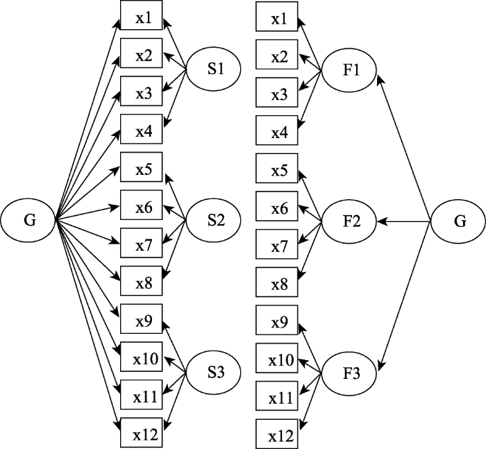
双因子模型又称为全局-局部因子模型(general-special factor model), 如图1中的M1所示。双因子模型假设同时存在全局因子(general factor)和局部因子(special factor), 全局因子解释所有题目的共同变异; 局部因子解释控制了全局因子后部分题目(测量了一个维度)的共同变异(Chen, et al., 2006; 顾红磊, 温忠麟, 2017)。该模型在很多领域都有应用, 如管理心理学、健康心理学、教育心理学等(Distefano, Greer, & Kamphaus, 2013; Howard, Gagné, Morin, & Forest, 2018; Wang, Fredricks, Hofkens, & Linn, 2016)。
图1
假设一份测验由m个题目${{x}_{1}},{{x}_{2}},\cdots ,{{x}_{m}}$组成, 测量了一个全局因子G和n个局部因子${{S}_{1}},{{S}_{2}},\cdots ,{{S}_{n}}$, 则题目${{x}_{i}}$可以表示为(叶宝娟, 温忠麟, 2012):
其中, ${{a}_{i}}$是题目xi在全局因子G上的负荷, ${{b}_{ij}}$是题目xi在局部因子Sj上的负荷, ${{\delta }_{i}}$是题目xi的测验误差。
该模型假设全局因子和局部因子不相关, 局部因子之间可以相关; 误差与全局因子、局部因子不相关, 且误差之间不相关。若局部因子之间也不相关, 则为正交双因子模型。和徐文一样, 本研究采用有3个局部因子、每个局部因子4个指标的正交双因子模型。
2.2 高阶因子模型
常见的高阶因子模型是二阶因子(second-order factor)模型, 如图1中的M2所示。高阶因子解释全部一阶因子(维度)的共同变异, 一阶因子解释相应维度的一组题目的共同变异(顾红磊, 温忠麟, 2017)。
假设一份测验由m个题目${{x}_{1}},{{x}_{2}},\cdots ,{{x}_{m}}$组成, 测量了一个高阶因子G和n个一阶因子${{F}_{1}},{{F}_{2}},\cdots ,{{F}_{n}}$, 则题目xi可以表示为(侯杰泰, 温忠麟, 成子娟, 2004):
其中, λij是题目xi在一阶因子Fj上的负荷, δi是题目xi的测验误差; hj是一阶因子Fj在高阶因子G上的负荷, Sj是一阶因子Fj被高阶因子G解释后的残差(简称为一阶因子的残差), 对应于双因子模型中的局部因子, 故两者都用符号S表示。该模型假设误差间不相关。本研究采用有3个一阶因子, 每个一阶因子4个题目的高阶因子模型。
2.3 两种模型的关系
高阶因子模型嵌套于双因子模型(Schmid & Leiman, 1957; Yung, et al., 1999), 任何一个高阶因子模型都可以转化为一个双因子模型。原来的高阶因子变成了全局因子, 一个题目xi在全局因子上的负荷ai等于该题目在一阶因子Fj上的负荷λij乘以该一阶因子在高阶因子上的负荷hj, 即ai = λijhj; 一阶因子Fj被高阶因子解释后的残差Sj变成了局部因子, 即一阶因子的残差相当于局部因子, 题目xi在局部因子Sj上的负荷就等于该题目在一阶因子上的负荷λij, 这不难将公式(3)代入公式(2)并与公式(1)比较推导出来(Demars, 2006; Schmid & Leiman, 1957)。
Schmid和Leiman (1957)证明在满足比例约束时, 两种模型是等价的。比例约束是指, 在每个维度中, 全局因子的负荷和局部因子的负荷之比等于一个常数, 此常数为一阶因子在高阶因子上的负荷hj, 但不同维度中这个常数可以不同。然而, 一般的双因子模型是不满足比例约束条件的, 实际中也很难找到多维构念恰好可用满足比例约束条件的双因子模型去拟合。例如, 在Personality and Individual Differences期刊发表的关于双因子模型应用的文章中, 有33篇论文报告了因子负荷, 没有一个双因子模型是满足比例约束的。
2.4 预测视角下两种模型的关系
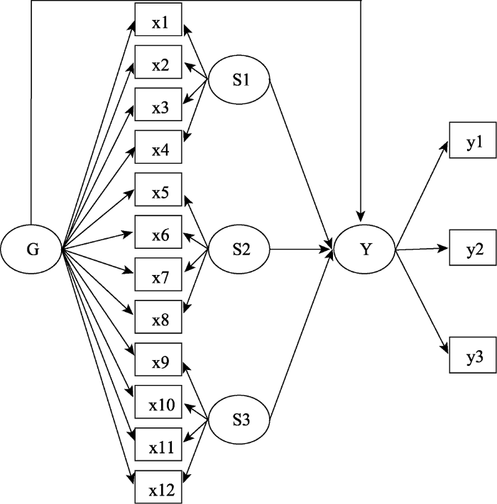
在双因子模型中, 全局因子作为预测变量表示所有题目的共同特质对效标的作用, 局部因子作为预测变量表示在控制了全局因子的影响后, 部分题目的额外共同特质对效标的作用, 如图2所示。当有n个局部因子时, 公式为
其中, c表示全局因子G对效标的效应大小, cj表示局部因子Sj对效标的效应大小, e表示预测残差。这里的效应就是所谓的结构系数。Mplus程序见附录1。
图2
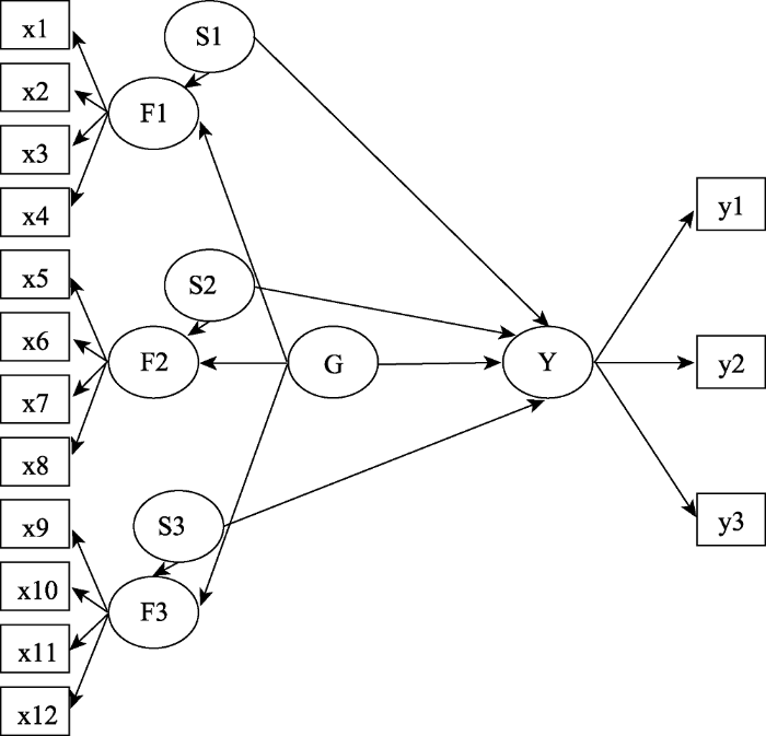
在高阶因子模型中, 虽然可以直接考虑高阶因子和一阶因子对效标的作用, 但为了跟徐文的相应模型一致, 先建立如下模型。在高阶因子模型中, 高阶因子作为预测变量表示一阶因子之间的共同特质对效标的作用, 一阶因子的残差(正是双因子模型的局部因子)作为预测变量表示部分题目的额外共同特质对效标的作用, 如图3所示。当有n个一阶因子时, 公式为
其中, c表示高阶因子G对效标的效应大小, cj表示一阶因子的残差Sj对效标的效应大小, e表示预测残差。
图3
对于上述高阶因子建模, EQS软件可以直接使用一阶因子的残差作为预测变量(Bentler, 1995), 但Mplus软件仅可以使用一阶因子作为预测变量(Muthén & Muthén, 2012)。把公式(3)代入公式(5)可得
根据公式(6), 可以将一阶因子作为预测变量, 其对效标的效应与一阶因子的残差作为预测变量时一模一样, 但此时高阶因子对效标的效应为$d=c-$ $\sum\limits_{j=1}^{n}{{{c}_{j}}}{{h}_{j}}$。因此, 在Mplus软件中, 可以把模型设置为高阶因子和一阶因子作为预测变量, 然后利用公式$c=d+\sum\limits_{j=1}^{n}{{{c}_{j}}}{{h}_{j}}$, 便可以转化为高阶因子和一阶因子的残差作为预测变量的结果。Mplus程序见附录2。
3 模拟研究
我们首先重复了徐文的模拟研究, 即真模型是满足比例约束的双因子模型。无论效标变量是显变量还是潜变量, 在估计偏差上得到的结果与徐文高度一致, 即满足比例约束的情形, 高阶因子模型结构系数的相对偏差比较小。此外还发现, 检验力方面, 若真模型是全局因子和局部因子同时作为预测变量, 整体上双因子模型的统计检验力较高。相应地, 无论真模型是全局因子还是局部因子作为预测变量, 都是高阶因子模型的第Ⅰ类错误率较小。为了节省篇幅, 这里不报告细节。
下面报告真模型为不满足比例约束的双因子模型的模拟研究, 这是徐文没有做的情形。虽然我们也考虑了效标为潜变量和显变量的两种设计, 但因为两种设计的结果高度一致, 所以下面只报告效标为潜变量的情形, 与徐文的一样, 效标潜变量有3个指标、标准化的负荷固定为比较有代表性的0.7 (也见Gu et al., 2017b)。模拟研究设计主要是针对预测变量的测量模型进行。
3.1 研究设计
真模型为不满足比例约束的双因子模型, 由符合下列条件的双因子模型Mb产生数据, 为与徐文对比, 参数设计尽量与徐文的设计一致, 但本文对结构系数也做了设计(在考虑用检验力和第I类错误率进行评价时是必须的)。
(1) 全局因子的负荷:0.4, 0.5, 0.6和0.7。全局因子共12个题目, 每种条件下, 全部12个题目在全局因子上的负荷都相等(Reise, Scheines, Widaman, & Haviland, 2013; 徐霜雪 等, 2017)。不满足比例约束条件的双因子模型的一个充分(但不必要)条件是, 不同题目在同一个局部因子上的负荷各不相等, 但在全局因子上的负荷相等。Mb每个局部因子的4个题目, 其负荷分别设置为0.4, 0.5, 0.6, 0.7。
(2) 全局因子和局部因子的结构系数设置了三种组合:0.3、0.3; 0、0.3; 0.3、0。例如, 0、0.3表示全局因子对效标的效应为0, 3个局部因子对效标的效应都是0.3。
(3) 样本容量: 200, 500和1000。
(4) 用于估计的模型:双因子模型Mb和高阶因子模型Mh。
本模拟实验是4×3×3×2的混合设计, 前3个因素都是被试间因素, 最后一个因素是被试内因素。对于被试间因素, 共有36种水平组合。使用Mplus 7.4模拟生成1000个样本数据, 即每种组合重复1000次。
全局因子负荷、局部因子负荷、结构系数、样本容量为条件, 估计的模型——双因子模型和高阶因子模型为关注对象。据此可以在不同数据条件下进行比较, 包括模型拟合程度、结构系数的相对偏差、统计检验力、第Ⅰ类错误率, 还可以了解当全局因子和局部因子负荷、样本容量变化时, 比较指标的变化。
3.2 结果
本文除了和徐文一样报告了样本容量为1000的结果外, 同时报告样本容量为500和200的结果。
3.2.1 适当解
排除不恰当解的结果, 如不收敛、方差和标准误为负的情形, 仅考虑恰当解的情况。样本容量为1000时, 两种模型的收敛率都在99%以上。随着样本容量减少, 两种模型的收敛率降低, 但都在92%以上, 最大相差6%。同种情况下, 高阶因子模型的收敛率高于双因子模型。
3.2.2 模型拟合
一般认为, CFI (comparative fit index)和TLI (Tucker-Lewis Index)大于0.9, RMSEA (Root Mean Square Error of Approximation)和SRMR (Standardized Root Mean square Residual)小于0.08, 则模型整体拟合良好(Marsh, Hau, & Wen, 2004; 温忠麟, 侯杰泰, 马什赫伯特, 2004)。信息指数AIC、ABIC越小, 则模型拟合越好(Burnham & Anderson, 1998)。所有条件下, 双因子模型拟合较好。虽然高阶因子模型拟合比双因子模型差, 但也达到了拟合良好的标准。
3.2.3 结构系数的相对偏差
相对偏差(relative bias)是指参数估计值的平均数和真实值之差除以真实值, 即$bias(\hat{c})=(mean(\hat{c})-$ $c)/c$, 用于衡量估计值的精度。一般认为, 相对偏差的绝对值在5%以内可以忽略(Hoogland & Boomsma, 1998), 在10%以内可以接受, 且可以认为是无偏估计(Reise et al., 2013)。和徐文一样, 本研究比较相对偏差的绝对值。
由于三个局部因子(一阶因子的残差)为预测变量时, 三条路径作用相同, 这里只考虑其中一条路径(S1因子的结构系数)的结果, 如图4所示。双因子模型结构系数的相对偏差比高阶因子模型的普遍较小, 但存在交互作用:样本容量较小而且全局因子负荷较低时, 双因子模型结构系数的相对偏差较大; 样本容量较大时, 双因子模型结构系数的相对偏差较小。85%的处理中, 双因子模型结构系数的相对偏差小于10%。随着样本容量的增加, 整体上两种模型结构系数的相对偏差变小。此外, 全局因子负荷越大, 双因子模型结构系数的相对偏差越小。
图4
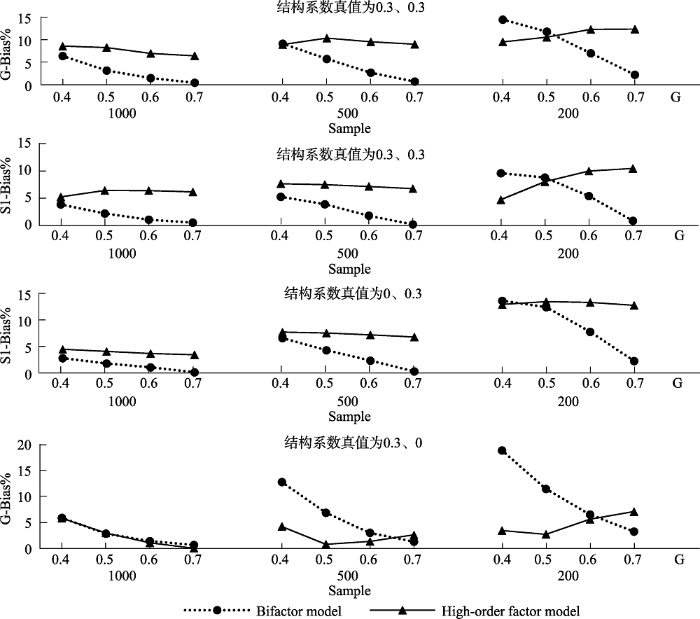
图4
不满足比例约束条件时结构系数的相对偏差
注:横轴G表示全局因子负荷(下同); 纵轴G-Bias%表示G因子的结构系数的相对偏差; S1-Bias%表示S1因子的结构系数的相对偏差。
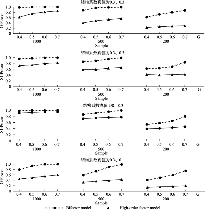
3.2.4 统计检验力
统计检验力(power)是指真值不为0时, 估计值显著不等于0的概率。统计检验力越接近1越好。由图5可见, 在所有条件下, 都是双因子模型的统计检验力比较高。样本容量越大, 两种模型的统计检验力都越高。此外, 全局因子负荷越大, 两种模型的统计检验力都越高。
图5
3.2.5 第I类错误率
第I类错误率(type I error rate)是指真值为0时, 估计值显著不等于0的概率。一般认为第I类错误率越接近真值0.05越好, 在0.025~0.075之间是可以接受的(Bradley & James, 1978; Mackinnon, Lockwood, & Williams, 2004; Wu et al., 2013)。
和检验力的结果类似, 双因子模型的第I类错误率比较大(见图6)。当N = 1000时, 在模拟的各种条件下两种模型的第I类错误率几乎都在可接受范围。但在样本容量较小而且全局因子负荷较低时, 双因子模型的第I类错误率大于可接受的范围。全局因子负荷越大, 双因子模型的第I类错误率越接近0.05。
图6

图6
不满足比例约束条件时结构系数的第I类错误率
注:G-I Error表示G因子的结构系数的第I类错误率, S1-I Error表示S1因子的结构系数的第I类错误率。
3.3 小结
本模拟研究是徐文没做的一个新研究, 产生数据的双因子模型不等价于任何一个高阶因子模型。多数情况下, 双因子模型结构系数的相对偏差比较小, 尤其是当N = 1000的时候, 双因子模型一致小于高阶因子模型。但在N小的时候, 两种模型的相对偏差大小比较没有一致的结果, 尤其是全局因子的负荷较小时。检验力方面, 各种情况下都是双因子模型的比较高。相应地, 无论真模型是全局因子还是局部因子作为预测变量, 都是双因子模型的第I类错误率比较大。
4 结论和讨论
徐文研究以满足比例约束的双因子模型(此时等价于一个高阶因子模型)为真实测量模型产生模拟数据, 比较了用双因子模型和高阶因子模型作为测量模型的结构系数。在其研究中, 无论使用的是双因子模型还是高阶因子模型, 都是拟合了真模型。本文使用不满足比例约束的双因子模型为真实测量模型产生模拟数据进行比较, 无论结果是否与徐文相同, 都是有意义的。徐文的模拟研究结果只能说明, 满足比例约束条件时, 高阶因子模型结构系数的相对偏差更小。但一般情况下比例约束条件是不满足的, 在此种情况下, 如果徐文的结果还正确, 则可将徐文结果推广到很一般的范围; 如果徐文结果不再正确, 则本文的意义更大。此外, 本文从多角度比较了两种模型的表现, 包括拟合指数、结构系数的相对偏差、统计检验力、第I类错误率。
当真模型满足比例约束条件时, 与双因子模型相比, 高阶因子模型结构系数的相对偏差较小(这和徐文的结果一致); 第I类错误率较低, 但检验力也较低。两种模型的拟合程度差别不大, 都达到拟合良好的标准。考虑到高阶因子模型比较省检(自由度更大), 当模型满足或近似满足比例约束条件时, 首选高阶因子模型进行预测, 尤其是样本容量较大时, 检验力较低的缺点会消失。
当真模型不满足比例约束条件时, 使用高阶因子模型可以说是拟合了误设模型。即使高阶因子模型的拟合指数还是可以接受, 但比双因子模型拟合要差。更重要的是, 与高阶因子模型相比, 双因子模型结构系数的相对偏差普遍较小, 尤其是当N较大的时候。这与徐文的结果正好相反, 所以徐文的结果没有普遍性。此外, 各种情况下都是双因子模型的统计检验力较高, 相应地, 第I类错误率也略高(尤其样本容量比较小的时候)。总之, 当模型不满足比例约束条件时(通常的应用属于此种情况), 从统计角度不能说高阶因子模型比双因子模型还好。
那么, 是不是在预测视角下, 就优先考虑双因子模型呢?也不是, 而是应当从学科理论出发、结合研究目的选用模型。与双因子模型相比, 高阶因子模型不仅更加简洁, 而且其中的一阶因子比局部因子更容易理解。如果研究者使用高阶因子模型进行预测, 而整个模型已经拟合良好, 且各项评价指标也达到要求, 是可以接受的。但高阶因子模型可以接受, 并不能说它优于双因子模型。
高阶因子模型的高阶因子定义在一阶因子上而非观测变量(题目)上, 因此高阶因子对观测变量没有直接效应, 一阶因子相当于中介变量, 高阶因子对观测变量的作用完全通过一阶因子的作用实现(Gignac, 2008; 顾红磊, 温忠麟, 2017)。而双因子模型的全局因子和局部因子都直接定义在观测变量上, 对观测变量都是直接效应, 有时候更易解释全局因子、局部因子和效标变量之间的关系(Beaujean, Parkin, & Parker, 2014; Chen et al., 2006)。特别是当使用高阶因子模型结果不理想的时候, 双因子模型是值得考虑的替代模型。
本研究中发现若不满足比例约束条件, 样本容量为1000时, 双因子模型的第I类错误率基本上可以接受; 样本容量为500时, 近六成的处理中双因子模型的第I类错误率都在可接受的范围内。因此, 使用双因子模型时样本宜大一些, 比如不小于500。此外, 高阶因子模型尤其是双因子模型较难收敛, 样本容量越大越有助于提高收敛性, 而且大样本(如超过500)得到的预测偏差基本上在可接受范围, 也有较高的检验力。
有时候根据常用的拟合指数可能不知道是用双因子模型还是高阶因子模型拟合多维构念较好, 但模拟研究发现满足比例约束的双因子模型和不满足比例约束的双因子模型的信息指数(例如, AIC、ABIC)表现不一。对于AIC和ABIC, 满足比例约束条件时双因子模型的比较大, 而不满足比例约束条件时高阶因子模型的比较大。在实证研究中, 可以通过比较两种模型的AIC和ABIC判断哪个更适宜拟合多维构念。如果双因子模型的AIC、BIC较大, 倾向于选用高阶因子模型, 否则考虑使用双因子模型研究结构系数, 也便于进一步解释多维构念与效标之间的关系。
为了比较徐文结果, 本研究与徐文一样使用正交双因子模型。但正交双因子模型假设局部因子间不相关。在更一般的情况下, 即双因子模型的局部因子允许相关, 本研究结果是否全部成立, 有待进一步研究。
附录1
TITLE: Bifactor model
DATA: FILE = p1.dat; !文件名
VARIABLE: NAMES = y1-y3 x1-x12; !变量命名
MODEL:
Y by y1-y3; !Y表示效标变量
S1 by x1-x4*;
S2 by x5-x8*;
S3 by x9-x12*; !S1-S3表示局部因子
G by x1-x12*;!G表示全局因子
G@1; S1-S3@1; G with S1-S3@0; S1-S3 with S1- S3@0;
Y ON G S1-S3;!全局因子和局部因子作为预测变量
OUTPUT: stdyx;
附录2
TITLE: High-order factor model
DATA: FILE = p1.dat; !文件名
VARIABLE: NAMES = y1-y3 x1-x12;!变量命名
MODEL:
Y by y1-y3; !Y表示效标变量
F1 by x1-x4;
F2 by x5-x8;
F3 by x9-x12; !F1-F3表示一阶因子
G by F1-F3*(h1-h3);!G表示高阶因子
G@1; F1-F3@1;
Y ON G*(d)
F1-F3*(c1-c3);!高阶因子和一阶因子作为预测变量
MODEL CONSTRAINT:
NEW (c); !c为高阶因子和一阶因子的残差作为预测变量时, 高阶因子的结构系数。
c=d+h1*c1+h2*c2+h2*c2;
OUTPUT: stdyx ;
参考文献
Comparing Cattell-Horn-Carroll factor models: Differences between bifactor and higher order factor models in predicting language achievement
DOI:10.1037/a0036745
URL
PMID:24840178

Abstract Previous research using the Cattell-Horn-Carroll (CHC) theory of cognitive abilities has shown a relationship between cognitive ability and academic achievement. Most of this research, however, has been done using the Woodcock-Johnson family of instruments with a higher order factor model. For CHC theory to grow, research should be done with other assessment instruments and tested with other factor models. This study examined the relationship between different factor models of CHC theory and the factors' relationships with language-based academic achievement (i.e., reading and writing). Using the co-norming sample for the Wechsler Intelligence Scale for Children--4th Edition and the Wechsler Individual Achievement Test--2nd Edition, we found that bifactor and higher order models of the subtests of the Wechsler Intelligence Scale for Children-4th Edition produced a different set of Stratum II factors, which, in turn, have very different relationships with the language achievement variables of the Wechsler Individual Achievement Test--2nd Edition. We conclude that the factor model used to represent CHC theory makes little difference when general intelligence is of major interest, but it makes a large difference when the Stratum II factors are of primary concern, especially when they are used to predict other variables. PsycINFO Database Record (c) 2014 APA, all rights reserved.
EQS 6 structural equations program manual.
Robustness?
Model selection and inference: A practical information-theoretic approach.
Modeling general and specific variance in multifaceted constructs: A comparison of the bifactor model to other approaches
DOI:10.1111/j.1467-6494.2011.00739.x
URL
PMID:22092195
[本文引用: 1]
This article recommends an alternative method for testing multifaceted constructs. Researchers often have to choose between two problematic approaches for analyzing multifaceted constructs: the total score approach and the individual score approach. Both approaches can result in conceptual ambiguity. The proposed bifactor model assesses simultaneously the general construct shared by the facets and the specific facets, over and above the general construct. We illustrate the bifactor model by examining the construct of Extraversion as measured by the Revised NEO Personality Inventory (NEO-PI-R; Costa & McCrae, 1992), with two college samples (N65=65383 and 378). The analysis reveals that the facets of the NEO-PI-R Extraversion correlate with criteria in opposite directions after partialling out the general construct. The direction of gender differences also varies by facets. Bifactor models combine the advantages but avoid the drawbacks of the 2 existing methods and can lead to greater conceptual clarity.
Two concepts or two approaches? A bifactor analysis of psychological and subjective well-being
DOI:10.1007/s10902-012-9367-x
URL
AbstractResearchers often debate about whether there is a meaningful differentiation between psychological well-being and subjective well-being. One view argues that psychological and subjective well-being are distinct dimensions, whereas another view proposes that they are different perspectives on the same general construct and thus are more similar than different. The purpose of this investigation was to examine these two competing views by using a statistical approach, the bifactor model, that allows for an examination of the common variance shared by the two types of well-being and the unique variance specific to each. In one college sample and one nationally representative sample, the bifactor model revealed a strong general factor, which captures the common ground shared by the measures of psychological well-being and subjective well-being. The bifactor model also revealed four specific factors of psychological well-being and three specific factors of subjective well-being, after partialling out the general well-being factor. We further examined the relations of the specific factors of psychological and subjective well-being to external measures. The specific factors demonstrated incremental predictive power, independent of the general well-being factor. These results suggest that psychological well-being and subjective well-being are strongly related at the general construct level, but their individual components are distinct once their overlap with the general construct of well-being is partialled out. The findings thus indicate that both perspectives have merit, depending on the level of analysis.
A comparison of bifactor and second-order models of quality of life
DOI:10.1207/s15327906mbr4102_5
URL
PMID:26782910
[本文引用: 1]
Bifactor and second-order factor models are two alternative approaches for representing general constructs comprised of several highly related domains. Bifactor and second-order models were compared using a quality of life data set (N = 403). The bifactor model identified three, rather than the hypothesized four, domain specific factors beyond the general factor. The bifactor model fit the data significantly better than the second-order model. The bifactor model allowed for easier interpretation of the relationship between the domain specific factors and external variables, over and above the general factor. Contrary to the literature, sufficient power existed to distinguish between bifactor and corresponding second-order models in one actual and one simulated example, given reasonable sample sizes. Advantages of bifactor models over second-order models are discussed.
The bifactor model fits better than the higher-order model in more than 90% of comparisons for mental abilities test batteries
DOI:10.3390/jintelligence5030027 URL
Application of the bi-factor multidimensional item response theory model to testlet- based tests
DOI:10.1111/j.1745-3984.2006.00010.x
URL
Four item response theory (IRT) models were compared using data from tests where multiple items were grouped into testlets focused on a common stimulus. In the bifactor model each item was treated as a function of a primary trait plus a nuisance trait due to the testlet; in the testlet-effects model the slopes in the direction of the testlet traits were constrained within each testlet to be proportional to the slope in the direction of the primary trait; in the polytomous model the item scores were summed into a single score for each testlet; and in the independent-items model the testlet structure was ignored. Using the simulated data, reliability was overestimated somewhat by the independent-items model when the items were not independent within testlets. Under these nonindependent conditions, the independent-items model also yielded greater root mean square error (RMSE) for item difficulty and underestimated the item slopes. When the items within testlets were instead generated to be independent, the bi-factor model yielded somewhat higher RMSE in difficulty and slope. Similar differences between the models were illustrated with real data.
Multifactor modeling of emotional and behavioral risk of preschool-age children
DOI:10.1037/a0031393
URL
PMID:23356680
Screening for emotional and behavioral risk has become more prevalent with young children; however, not much is known about the latent structure for many of the brief instruments currently being used to assess children. Information concerning the latent structure of an instrument is necessary to support use of the scoring information. The underlying structure of the Behavioral and Emotional Screening System, Teacher Rating Form-Preschool (Kamphaus & Reynolds, 2007) was investigated. A sample of ratings of more than 1,400 preschoolers was used to test 4 different confirmatory factor analysis models: (a) unidimensional model, (b) correlated factor model, (c) higher order factor model, and (d) bifactor model. Results showed support for the bifactor model, suggesting that an overall score is useful for interpreting preschoolers' level of emotional and behavioral risk. Relationships between items and the maladaptive risk general factor varied according to content area.
Higher-order models versus direct hierarchical models: A superordinate or breadth factor?
Reporting and interpreting multidimensional test scores: A bi-factor perspective
多维测验分数的报告与解释: 基于双因子模型的视角
在心理、行为、管理和教育等社科领域,经常使用多维测验。本文评介并比较了各种多维测验的测量模型;总结了基于双因子模型计算得到的统计指标;根据不同研究目的,提出了两个兼顾简洁性和精确性的多维测验分析流程。作为例子,在马基雅维利主义人格量表的研究中,通过双因子模型分析了如何报告、解释多维测验分数以及如何利用多维建模进行后续分析。
Structural validity of the Machiavellian personality scale: A bifactor exploratory structural equation modeling approach
DOI:10.1016/j.paid.2016.09.042
URL
61The bifactor ESEM model provided the best fit to the MPS data.61The Machiavellian Personality Scale was dominated by the global Machiavellianism.61It is suggested to report the total score and thedesire for controlsubscale score when using the MPS in practice.
Examining and controlling for wording effect in a self-report measure: A Monte Carlo simulation study
DOI:10.1080/10705511.2017.1286228
URL
(2017). Examining and Controlling for Wording Effect in a Self-Report Measure: A Monte Carlo Simulation Study. Structural Equation Modeling: A Multidisciplinary Journal. Ahead of Print. doi: 10.1080/10705511.2017.1286228
General and specific abilities as predictors of school achievement
DOI:10.1207/s15327906mbr2804_2 URL
Structural equation model and its applications
结构方程模型及其应用
Robustness studies in covariance structure modeling: An overview and a meta- analysis
Using bifactor exploratory structural equation modeling to test for a continuum structure of motivation
A bifactor approach to modelling the Rosenberg Self Esteem Scale
DOI:10.1016/j.paid.2014.03.034
URL
[本文引用: 1]
Inconsistency exists in the empirical literature with respect to the underlying factor structure of the Rosenberg Self-Esteem Scale (RSES; Rosenberg, 1989). In research contexts the RSES is considered a unidimensional measure of self-esteem. Empirical findings have undermined this conceptualisation with factor analytic findings favouring a variety of one-factor solutions (with correlated measurement errors) or multidimensional representations. The current study applied a bifactor modelling approach to provide a theoretical and methodologically satisfying resolution to the current inconsistency. Three alternative factor models of the RSES were tested among a large sample of the adult population (N=6082). Results indicated that a bifactor model was the best fit of the data. This model was demonstrated to be factorially invariant among males and females. The reliability of the scale was established using composite reliability. Results are discussed in terms of resolving the debate about the appropriate factor structure of the RSES.
Confidence limits for the indirect effect: Distribution of the product and resampling methods
DOI:10.1207/s15327906mbr3901_4 URL
In search of golden rules: Comment on hypothesis-testing approaches to setting cutoff values for fit indexes and dangers in overgeneralizing Hu and Bentler's (1999) findings
DOI:10.1207/s15328007sem1103_2
URL
Goodness-of-fit (GOF) indexes provide "rules of thumb" ecommended cutoff values for assessing fit in structural equation modeling. Hu and Bentler (1999) proposed a more rigorous approach to evaluating decision rules based on GOF indexes and, on this basis, proposed new and more stringent cutoff values for many indexes. This article discusses potential problems underlying the hypothesis-testing rationale of their research, which is more appropriate to testing statistical significance than evaluating GOF. Many of their misspecified models resulted in a fit that should have been deemed acceptable according to even their new, more demanding criteria. Hence, rejection of these acceptable-misspecified models should have constituted a Type 1 error (incorrect rejection of an "acceptable" model), leading to the seemingly paradoxical results whereby the probability of correctly rejecting misspecified models decreased substantially with increasing N. In contrast to the application of cutoff values to evaluate each solution in isolation, all the GOF indexes were more effective at identifying differences in misspecification based on nested models. Whereas Hu and Bentler (1999) offered cautions about the use of GOF indexes, current practice seems to have incorporated their new guidelines without sufficient attention to the limitations noted by Hu and Bentler (1999).
Mplus user’s guide (7 th ed.).
Multidimensionality and structural coefficient bias in structural equation modeling: A bifactor perspective
DOI:10.1177/0013164412449831 URL [本文引用: 1]
Competing factor structures of the Rosenberg Self-Esteem Scale (RSES) and its measurement invariance across clinical and non-clinical samples
DOI:10.1016/j.paid.2017.02.063
URL
Although several studies have investigated the factor structure of the Rosenberg Self-Esteem Scale (RSES), there are still disagreements about it. The present study assessed: a) the goodness of fit of nine competing factor models for the RSES using data from a clinical sample of 855 women with eating/weight disorders; and b) its measurement invariance across clinical and non-clinical (n = 943) samples. A bifactor model, with a general self-esteem factor, plus positive and negative method factors, provided a better fit with the data than alternative models. However, the results showed the high reliability of the general self-esteem factor, and a low reliability of the two method factors. Furthermore, the full metric invariance of the RSES, as well as a partial scalar invariance and partial strict invariance across clinical and non-clinical groups, was supported by our findings. The factor variances and means differed significantly across groups. Overall, the findings of this study showed that the factor structure of the RSES is contaminated by method effects due to item wording, also with clinical samples, and that respondents from clinical and non-clinical groups interpret the self-esteem construct of the RSES items in a substantially similar way.
The development of hierarchical factor solutions
The math and science engagement scales: Scale development, validation, and psychometric properties
DOI:10.1016/j.learninstruc.2016.01.008
URL
61Developing appropriate instruments to measure student engagement in math and science is needed.61Student engagement is a multidimensional construct, including behavioral, emotional, cognitive, and social components.61The use of multiple informants to assess student engagement provides a more comprehensive perspective.61Math and science engagement predicted academic performance and career aspirations.
Structural equation model testing: Cutoff criteria for goodness of fit indices and chi-square test
结构方程模型检验:拟合指数与卡方准则
讨论了Hu和Bentler(1998,1999)推荐的检验结构方程模型的 7个拟合指数准则 ,对这 7个指数的历史、特点和表现做了比较详细的述评。指出了他们基于这 7个指数的单指数准则和 2 -指数准则的不足之处。提出了超低显著性水平下的卡方准则 ,并部分重复他们的模拟例子 ,将卡方准则与这 7个指数准则比较 ,结果说明新的卡方准则优于其中的 6个 ,与另一个相当。最后简要说明了应当如何检视拟合指数进行模型检验和模型比较。
A comparison of strategies for forming product indicators for unequal numbers of items in structural equation models of latent interactions
DOI:10.1080/10705511.2013.824772
URL
[本文引用: 1]
This Monte Carlo simulation study investigated different strategies for forming product indicators for the unconstrained approach in analyzing latent interaction models when the exogenous factors are measured by unequal numbers of indicators under both normal and nonnormal conditions. Product indicators were created by (a) multiplying parcels of the larger scale by items of the smaller scale, and (b) matching items according to reliability to create several product indicators, ignoring those items with lower reliability. Two scaling approaches were compared where parceling was not involved: (a) fixing the factor variances, and (b) fixing 1 loading to 1 for each factor. The unconstrained approach was compared with the latent moderated structural equations (LMS) approach. Results showed that under normal conditions, the LMS approach was preferred because the biases of its interaction estimates and associated standard errors were generally smaller, and its power was higher than that of the unconstrained approach. Under nonnormal conditions, however, the unconstrained approach was generally more robust than the LMS approach. It is recommended to form product indicators by using items with higher reliability (rather than parceling) in the matching and then to specify the model by fixing 1 loading of each factor to unity when adopting the unconstrained approach.
Simulated data comparison of the predictive validity between bi-factor and high-order models
预测视角下双因子模型与高阶模型的模拟比较
DOI:10.3724/SP.J.1041.2017.01125
URL
[本文引用: 1]
双因子模型和高阶因子模型,作为既有全局因子又有局部因子的两个竞争模型,在研究中得到了广泛应用。本文采用Monte Carlo模拟方法,在模型拟合比较的基础上,比较了效标分别为外显变量和内潜变量时,两个模型在各种负荷水平下预测准确度的差异。结果发现,两种模型在拟合效果方面无显著差异;但在预测效度方面,当效标为显变量时,两个模型的结构系数估计值皆为无偏估计;而效标为潜变量时,高阶因子模型表现优于双因子模型:高阶因子模型的结构系数为无偏估计,双因子模型的结构系数估计值则在50%左右的情况下存在偏差。
Estimating homogeneity coefficient and its confidence interval
测验同质性系数及其区间估计
DOI:10.3724/SP.J.1041.2012.01687
URL
[本文引用: 1]
Multidimensional tests are frequently applied to the studies of psychology, education, society and management. Before aggregating all item scores to form a composite score of a multidimensional test, we should consider the homogeneity of the test. Homogeneity coefficient which reflects the extent that all test items measure the same trait can be employed to evaluate test homogeneity. If homogeneity coefficient is low, the composite score is meaningless and cannot be used for further analyses. Homogeneity coefficient is the proportion of variability in composite score that is accounted for by the general factor, which is viewed as common to all items. Any multidimensional test can be represented by a bifactor model that contains a general factor and local factors. Hence homogeneity coefficient can be calculated based on a bifactor model. A unidimensional test with positively worded items and negatively worded items can also be represented by a bifactor model, where the assessed construct is the general factor and method factors are local factors. The confidence interval of homogeneity coefficient provides more information than its point estimate. There are three approaches to estimate the confidence interval of composite reliability: Bootstrap method, Delta method and direct use of the standard error generated from an SEM software output (e.g., LISREL). It has been found that the interval estimates that obtained by Delta method and Bootstrap method were almost the same, whereas the results obtained by LISREL software and by Bootstrap method had large differences. Delta method was recommended when estimating the confidence interval of composite reliability. In order to compute the confidence interval of homogeneity coefficient, we deduced a formula by using Delta method for computing the standard error of homogeneity coefficient. Based on the standard error, the confidence interval can be obtained easily. We used an example to illustrate how to calculate homogeneity coefficient and its confidence interval by using the proposed Delta method with LISREL software. We also illustrated how to get the same result with Mplus software that automatically calculates the standard error with Delta method and presents the confidence interval. Before composite scores of a test are aggregated for further statistical analysis, it is recommended to report homogeneity coefficient so that readers could evaluate the extent that the statistical results are reliable.
On the relationship between the higher-order factor model and the hierarchical factor model
DOI:10.1007/BF02294531
URL
[本文引用: 1]
The relationship between the higher-order factor model and the hierarchical factor model is explored formally. We show that the Schmid-Leiman transformation produces constrained hierarchical factor...
