

传统的分析方法多以变量为分析对象, 例如因素分析(factor analysis, FA)将条目分成不同的因子或维度。近年来以个体为中心(person-centered)的方法逐渐引起心理学研究者的兴趣。其中潜类别分析(latent Class Analysis, LCA)和潜剖面分析(Latent Profile Analysis, LPA)是个体为中心分析方法中最基本也是最常用的分析方法(邱皓政, 2008; Collins & Lanza, 2010)。LCA在心理学、预防医学、精神病学、市场营销、组织管理等诸多领域已广为使用(e.g., 张洁婷, 焦璨, 张敏强, 2010)。
通常, 将LCA和FA作为测量模型, 因为两者都是处理潜变量和测量指标间关系的统计模型。与FA不同, LCA根据个体在观测指标上的作答反应将其归入特定的潜类别组(latent class)。然而LCA同FA一样, 也可以进一步拓展, 纳入协变量(预测变量和结果变量)。纳入协变量的FA即结构方程模型(Structure Equation Model, SEM); 纳入协变量的LCA称作带有协变量的潜类别模型以及更一般的形式——回归混合模型(Regression Mixture Modeling, RMM; e.g., Clark &MuthÉn, 2009)。例如, 考察性别、种族等人口学变量对潜类别分组的影响。本文首先对近年来提出的处理带有协变量的潜类别模型的新方法进行逐一介绍; 同时以一个具体的分析实例演示不同处理方法的分析过程。文章最后对当前研究存在的问题和将来的发展趋势进行简要评价。
1 潜类别模型
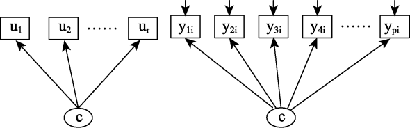
潜在类别分析或潜类别模型是通过类别潜变量来解释外显指标间的关联, 使外显指标间的关联通过潜在类别变量来估计, 进而维持其局部独立性(local independence)的统计方法(见图1) (邱皓政, 2008; Collins & Lanza, 2010)。其基本假设是, 外显变量各种反应的概率分布可以由少数互斥的潜在类别变量来解释, 每种类别对各外显变量的反应选择都有特定的倾向(邱皓政, 2008; Collins & Lanza, 2010)。与潜在类别分析非常相似的是潜在剖面分析, 区别在于前者处理分类变量, 后者分析连续变量。
图1
可以从方差分析的角度理解LCA。方差分析的特点是将方差分解成不同的来源, 常见的有组间vs.组内和被试间vs.被试内。在LCA中, 可以将方差分解为类别内和类别间(Sterba, 2013)。
根据局部独立性假设, 类别内的任意两个观测指标间的关联已通过潜类别变量解释, 所以它们之间已没有关联。根据独立事件联合发生的概率等于单独发生概率之积的原理, 在每个类别内部, 多个两点计分项目的联合概率可以表示为:
上式中, ${{Y}_{i}}$表示个体i在指标j的两个选项y = 1或y = 0的得分。下标j表示2点计分的指标, c为潜类别变量, 有k个水平。
同时考虑多个类别水平时, 上式扩展为:
$p\left( {{c}_{i}}=k \right)$表示某一类别组k所占总体的比率, 亦称潜类别概率。
2 带有协变量的潜类别模型
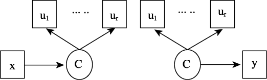
在应用研究中, 研究者往往不仅关心将个体划分到特定的潜类别组, 而且希望探索哪些变量可以预测个体的潜类别分组或不同的潜类别分组如何预测重要的结果变量。这两种情况分别对应包含预测变量(predictor variable)的LCA和包含结果变量(outcome variable或distal variable)的LCA, 如图2所示。在左图中, 类别潜变量C由测量指标U测量; 左图中预测变量X指向类别潜变量C的箭头表示协变量影响个体类别归属。例如, 某研究试图了解人口学变量对儿童行为问题潜类别归属的影响, 根据5个测量儿童行为问题的指标将450名儿童分成4个潜类别组(即潜类别变量“问题行为”有4个水平), 然后做人口学变量(性别, 家庭经济地位和年龄等)对潜类别变量的回归模型。在右图中, 箭头的方向从潜类别变量C指向结果变量y, 表示类别属性(分类变量)预测结果变量。假设儿童问题行为潜类别归属可能会影响儿童学习成绩。由于成绩通常是连续变量, 所以此时为线性回归。也可以理解为不同问题行为类别的儿童学习成绩存在差异, 根据类别潜变量将儿童分成4组然后做方差分析。此时方差分析和线性回归等价。
图2
在回归模型中, 通常是根据因变量的类型选择对应的回归模型。左图中, 类别变量C通常有2个及以上水平, 因此logistic回归和多项logistic回归是最常见的分析模型。右图的回归类型较为多样,主要取决于y变量的类型, 可能是线性回归也可能是其他形式的回归模型。下面的介绍包含了两种不同协变量LCA的分析方法。
2.1包含预测变量的潜类别模型
总的来说, 带有预测变量的LCA的建模策略可以大致分成2大类:单步法和分步法(三步法)。顾名思义, 单步法在建模时一步完成所有模型(测量和结构)参数估计; 而分步法则采用逐步建模的步骤完成参数估计。
(1)单步法
单步法(one-step method)在处理带有协变量的LCA时, 同时完成潜类别分组(测量模型部分)和协变量关系建模(结构模型部分)。如果协变量是预测变量, 将其直接纳入模型进行分析, 协变量与潜类别变量的关系在LCA分析中同步完成。考虑协变量时的LCA表达式:
$P\left( C=t\text{ }\!\!|\!\!\text{ }{{Z}_{i}} \right)$为考虑协变量Z时, 属于潜类别t的概率, 该值可通过多项式逻辑斯特回归获得(Bakk&Vermunt, 2016):
上式中的αt和βt分别表示类别特定的截距和斜率。
如果协变量是结果变量(图2右图), 只需将结果变量当作LCA的测量指标纳入模型(具体见后文)。然而单步法存在如下几点不足(Vermunt, 2010):
首先, 当存在较多协变量时, 单步法的实际操作性较差。在探索性研究中, 由于缺少相关研究或理论预期, 模型中常常包含多个预测变量。在单步法中, 不同协变量的纳入和剔除都会影响测量模型(LCA)的结果, 使得整个分析过程非常繁琐。
第二, 模型建模困难。混合模型建模过程中最重要也是最复杂的问题是潜类别个数的确定, 包含协变量使得这一过程更加复杂。
第三, 单步法在实践中不易为应用研究者理解和掌握。回归混合模型的逻辑顺序是先根据LCA将样本分组; 接着以分组(潜)类别变量作为观测自变量或因变量进行回归分析, 而在单步法中这些过程是一步完成的, 理解和解释上较为抽象。
第四, 包含协变量的LCA模型可能会违反混合模型的前提假设如协变量在类别内的方差相等或/和正态分布等(Bauer & Curran, 2003)。
由于单步法的上述困难和不足, 分析过程清晰的三步法受到方法学者和应用研究者的广泛关注(e.g., Morin, Morizot, Boudrias, &Madore, 2011)。
(2)简单三步法
按照大多数应用研究者的分析习惯, 在做混合模型(mixture modeling)1(1混合模型比LCA和LPA更具一般的形式。)分析时, 通常根据多个测量指标采用LCA将样本分成不同的潜类别组(测量模型部分)。然后将类别潜变量作为观测类别变量进行后续分析。常见的后续分析有:比较变量在潜类别组上的差异(独立样本t检验或方差分析); 其他变量预测类别潜变量或类别潜变量预测其它变量。
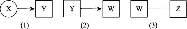
三步法的一般分析过程如图3所示:(1)进行常规的LCA模型估计, 这一步只使用LCA的测量指标; (2)接着在第一步的基础上根据后验概率获得个体的类别归属变量即潜类别分组变量; (3)最后将潜类别分组变量作为观测变量(分类变量)连同协变量进行回归分析。
图3
简单三步法也称作最可能类别回归法(Most Likely Class Regression; Clark &MuthÉn, 2009)2(2根据最大后验概率将个体分入到不同的潜类别组, 然后以该分组变量进行回归分析, 因此得名。)。这种方法符合应用研究者的分析习惯, 在实践中广为使用。
然而三步法也存在一些不足, 通常会低估类别潜变量和协变量的关系, 分类误差越大, 系数低估越明显(Bolck, Croon, &Hagenaars, 2004; Vermunt, 2010)。LCA分析的关键在于分类精确性。分类精确性对于个体中心的方法来说可以理解为测量信度或测量误差问题。如果分类误差较大, 把不属于某一类别的个体划分到该类别将会影响整个分析结果的准确性。针对简单三步法存在测量误差的问题, 近年来研究者提出了一些校正方法来减少分类误差产生的影响(Bakk, Tekle, &Vermunt, 2013; Lanza, Tan, & Bray, 2013; Vermunt, 2010), 下面将逐一详细介绍。
(3)概率回归法和加权概率回归法
这两种方法的分析过程与简单三步法类似, 也是分成三步。具体来说, 第一步依据观测指标将个体分类即执行LCA分析。第二步将个体的后验概率进行转换再做回归分析:(1)概率回归法将后验概率进行对数转换, 转换后的数值作为结果进行回归分析; (2)加权概率回归法则根据后验分类结果直接与协变量进行回归但采用后验概率进行加权。两种方法都考虑了分类的不确定性, 与简单三步法相比回归系数的结果相对较为准确, 但由于后验概率的估计本身也是存在误差的, 所以回归系数的显著性检验存在错误结论的可能(Clark &MuthÉn, 2009)。
(4)虚拟类别法
LCA根据一次分析的后验概率将个体分组, 这种做法存在抽样误差的问题3(3这里类似参数估计的点估计, 为了考虑抽样误差的影响通常采用区间估计。)。虚拟类别法(pseudoclass method, PC法)采用类似缺失值分析时使用的多重插补法, 从个体的后验概率分布中随机抽取若干个(通常20次)可能的后验概率值4(4因为存在分类不确定性所以抽取多个可能值作为分类误差。), 根据每次的概率值将个体分配到不同的类别, 然后平均若干次的结果作为最终的分类结果(Wang, Brown, &Bandeen-Roche, 2005)。
Clark和MuthÉn (2009)的模拟发现, 当分类精确性较高时(entropy > 0.8), 该方法表现较好; 然而在最近的模拟研究中发现, 与稳健三步法和单步法相比, 虚拟类别法在同等条件下表现最差 (Asparouhov&MuthÉn, 2014), 在实际应用中并不被推荐使用。
(5)稳健三步法或MML法
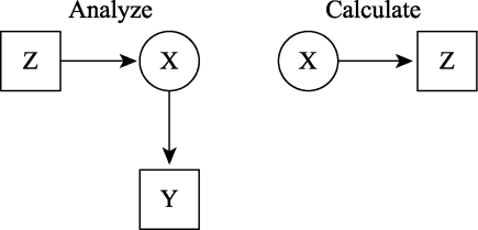
稳健三步法由Vermunt (2010)在Bolck等(2004)的研究基础上提出的。由于同时采用莫代尔分配法和极大似然估计, 因此又称作莫代尔极大似然估计法(Modal ML)。Asparouhov和MuthÉn (2014)将其称作三步法(3-steps approach), 为了区分简单三步法, 我们在这里将其称作稳健三步法。分析步骤同简单三步法, 区别在于第二步考虑了分类误差, 而简单三步法并未处理分类误差。稳健三步法5(5在Mplus中, 稳健三步法有两种实现形式:自动和手动。自动形式只需采用AUXILIARY的R3STEP选项, 软件自动完成上述3步分析。手动形式需要分别执行两步分析。第一步, 单独执行LCA分析, 获得分类错误率的对数形式。第二步, 在这一步分析中, 将第一步保留的分组变量N的均值固定为分类错误率的对数值。)的具体分析步骤如图4。
图4

图4
稳健三步法分析流程图(Asparouhov&MuthÉn, 2014)
稳健三步法最大的特点是在第二步考虑了分类误差或不确定性。假设W是基于模型估计的类别潜变量, 与实际的类别潜变量C并不完全一致(完全一致时不存在分类误差), 因此存在如下2个分类不确定率:
上式中, C为类别潜变量, N为根据后验分布概率将个体划分到不同潜类别组的变量(Mplus分析无条件LCA模型时保存后验概率后结果文件
的最后一列), U为观测指标。${{N}_{{{C}_{1}}}}$是根据N将个体划分到C1类别的数量。
在Mplus的新近版本中(7.2之后的版本),${{p}_{{{C}_{1}},{{C}_{2}}}}$的值可以在结果输出部分获得。随后可以计算“分类错误率”:$\text{ }\!\!~\!\!\text{ }P\left( N={{c}_{1}}\text{ }\!\!|\!\!\text{ }C={{c}_{2}} \right)$即实际属于C2类别但在LCA中根据后验概率却被归入C1的概率:
Nc是根据N将个体分配到C的数量。稳健三步法使用$\text{log}\left( {{q}_{{{c}_{1}},{{c}_{2}}}}/{{q}_{k,{{c}_{2}}}} \right)$作为N估计C的权重。
(6)修正的BCH法
BCH法最早由Bolck等(2004)提出, 用于处理包含分类预测变量的LCA。该方法与稳健三步法逻辑类似, 区别在于稳健三步法的第三步的估计方程采用极大似然估计, 而BCH将其转换成加权方差分析, 分类误差作为权重。
与稳健三步法相比, BCH法的一个突出优点是不会改变潜类别的顺序。潜类别顺序的改变是极大似然估计的一个“副产品”。由于ML估计常常得到局部最大化解而非整体最大化解, 所以混合模型估计通常设置多个起始值, 而起始值通常由软件随机生成, 所以每次分析的起始值不同得到的潜类别结果可能不同, 潜类别的顺序也可能不同。尽管使用相同的数据和指标, 所得到的拟合结果和类别数目也相同, 但类别潜变量水平的顺序可能不同(第一个类别变成第二个类别), 因此给潜类别分析带来很大的麻烦6(6 在稳健三步法分析中, Mplus自动监测顺序改变问题, 一旦发生顺序改变, Mplus将不报告结果(Asparouhov&Muthen, 2015)。)。
BCH法的不足在于, 当类别距离很小以及小样本量时, 类别内的误差方差可能是负值。此时如果把类别内方差固定相等, 也可以获得正确的类别组内结果变量的均值(Bakk&Vermunt, 2016)。
就目前的模拟研究结果来看, 稳健三步法和单步法是处理来有预测变量RMM最好的方法。根据通常的潜类别建模流程, 首先确定群体分类, 然后再在此基础上做进一步分析。稳健三步法的分析过程清晰明确, 符合广大应用研究者的分析习惯而容易被接受。
2.2包含结果变量的LCA
总的来说, 包含结果变量的LCA比包含预测变量的LCA要复杂一些, 因为在后者的建模过程中类别潜变量作为因变量只存在一种形式——logistic或多项式logistic回归。但在包含结果变量的LCA中, 结果变量存在两种形式:连续和类别变量。下面分别介绍两种不同形式结果变量的LCA分析方法。
2.2.1结果变量是连续变量
(1) 单步法
结果变量是连续变量时, 可以将结果变量当作LCA模型的指标, 同时完成模型估计。当局部独立性满足时, LCA表达式为公式2, 当纳入连续的协变量Z后, 公式2改写为联合的形式:
$f\left( {{Z}_{i}}\text{ }\!\!|\!\!\text{ }X=t \right)$为协变量Z在特定类别内的分布, 连续变量时为正态分布, 如果存在多个连续变量则为多元正态分布。
单步法需要满足重要的前提:连续结果变量在各类别内正态分布。如果正态假设不成立则会改变测量模型的结构及意义, 例如高估类别数(Bauer & Curran, 2003)。另外, 如果存在多个连续结果变量则更加复杂。假如采用每次只纳入一个结果变量的建模策略, 则会产生LCA模型混淆的问题:纳入不同结果变量间的LCA模型是不同的。
(2)LTB法
Lanza等(2013)最近提出了一种新的方法可以避免单步法违反假设时结果不准确的问题, 因为这种方法并没有特定的分布假设。在LTB法中, 首先将结果变量Z作为协变量纳入LCA分析(过程同包含预测变量的单步法), 流程如图5。
图5
第二步计算结果变量在每个类别内的均值(连续变量)或概率(类别变量)7(7自变量是分类变量(这里的潜类别变量)因变量是连续变量的回归模型等价于单因素方差分析。):
协变量Z在特定类别内的分布$f\left( Z\text{ }\!\!|\!\!\text{ }X=t \right)$可通过贝叶斯定理获得:
其中的$P\left( X=t\text{ }\!\!|\!\!\text{ }Z \right)$和$P\left( X=t \right)$是条件概率和类别概率由第一步获得。式中$f\left( Z \right)$未知, Asparouhov和MuthÉn (2014)建议使用Z的实证分布代替:
Lanza等(2013)并没有给出${{\mu }_{t}}$的标准误公式, Asparouhov和MuthÉn (2014)建议使用类别特定的方差的均方根除以类别特定的样本量获得, 但模拟研究发现这种做法会低估标准误(Bakk&Vermunt, 2016)。随后, Bakk, Oberski和Vermunt (2016)提出了Jackknife和Bootstrap再抽样的标准误。
当连续结果变量的方差在不同类别内相等时即同方差(homoskedastic errors), LTB法的估计结果是无偏的, 此时结果变量与潜类别变量之间呈linear-logistic关系。如果同方差不成立即异方差(heteroskedastic errors)时, LTB法估计类别特定的均值存在偏差(Bakk&Vermunt, 2016)。另外, LTB方法处理多个连续结果变量时存在困难, 如果采用分别建模的方式将面临单步法同样的困境。
(3)修正的LTB法
针对LTB法的不足, Bakk等(2016)结合稳健三步法的分析思想对LTB法进行了修正, 并将其分成三步实现, 因此这种方法与稳健三步法分析过程非常相似(流程见图6)。首先, 使用测量指标建立LCA, 同时根据后验概率将个体分到不同的潜类别组N。第二步, 考虑分类误差的前提下通过N估计潜类别变量C, 同时将结果变量Z作为协变量纳入分析(稳健三步法并未纳入协变量), 见公式11。
图6

上式中的$P\left( {{N}_{i}}=s\text{ }\!\!|\!\!\text{ }C=t \right)$被固定为上一步估计的N。
当连续结果变量的方差在不同类别内不相等时(类别内异方差), LTB法的估计结果是有偏的。
针对此问题, Bakk等(2016)提出在多项式逻辑斯特回归模型中加入二次项(公式12)来解决估计偏差的问题。
(4)修正BCH法
如前所述, BCH法8(8在Mplus里, 使用BCH分析包含结果变量RMM时非常方便, 只需一步即可实现, 例句见表2-8。)提出之初仅用于分析包含分类预测变量的LCA, 后来Vermunt (2010)对其进行了修正, 使其可以处理各种类型的变量。
(5)稳健三步法
稳健三步法也可以用于处理结果变量是连续变量的LCA。包含连续结果变量的LCA模型表达式变为:
$P\left( N=s\text{ }\!\!|\!\!\text{ }C=t \right)$被固定为第二步估计的分类精确性参数, $f\left( {{Z}_{i}}\text{ }\!\!|\!\!\text{ }C=t \right)$通常服从正态分布。如前所述, 结果变量是连续变量的LCA的目的在于估计结果变量在潜类别不同水平上的均值差异, 但结果变量的方差在不同类别组内可能相等也可能存在差异(类似方差分析时的组内方差同质假设)。针对方差的不同情况, 稳健三步法有两种不同的变式:类别组内方差同质和类别组内方差异质。
模拟研究发现(Bakk et al., 2013; Lanza et al., 2013), 当满足假设条件时9(9 ML和BCH假设连续结果变量在类别内的分布为正态分布。), 稳健三步法, BCH和LTB均可以得到无偏的参数估计结果(即类别特定的结果变量的均值)。然而, 当条件不成立时(非正态、方差不同质), 稳健三步法和LTB表现较差, 而BCH法则表现的很稳健(Bakk&Vermunt, 2016)。Asparouhov和MuthÉn (2015)通过模拟进一步比较了稳健三步法的两种变式(即类别等方差和类别不等方差; 分别对应Mplus中的DE3STEP和DU3STEP), LTB法, 单步法, PC法和BCH法在连续结果变量非正态(双峰分布)时的表现, 结果进一步证实了BCH的稳健性(其他方法表现均不佳)。尽管如此, 当类别距离或分类精确性较小时(比如entropy = 0.5), BCH也会低估标准误。他们的结果还发现, 当组内方差同质性不成立时, 方差不等的稳健三步法(DU3STEP)和BCH法表现最佳, 且前者更优。
2.2.2结果变量是类别变量
LTB法在处理分类结果变量时表现较好, 不会像分析连续结果变量时出现违反正态和方差同质假设后的估计偏差问题。在Asparouhov和MuthÉn (2014)的模拟研究中, 检验了3个样本量(N = 200, 500和2000)和2种分类精确性(entropy= 0.5和0.65)下LTB的表现, 结果发现仅在N = 200和entropy = 0.5时才会出现明显的偏差。
2.3回归混合模型方法的适用情境汇总表
为了方便读者对上述介绍的各种方法间的比较和选择, 在Asparouhov和MuthÉn (2015)的基础上, 表1汇总了带有不同协变量LCA分析方法的使用条件和简要评价, 以便研究者选用。
表1 各种情况处理方法汇总表
| 适用情况 | 方法 | Mplus语句: Auxiliary=() | 评价 | |
|---|---|---|---|---|
| 结果变量 | 分类 变量 | 单步法 | 无单独语句 | 直接将类别结果变量作为LCA的测量指标; 这种做法显然会影响测量模型; 纳入不同的结果变量会造成测量模型结果的差异, 因此不推荐使用。 |
| LTB | DCAT | 是处理类别结果变量最好的方法之一, 推荐使用。 | ||
| 连续 变量 | 单步法 | 无单独语句 | 非正态时表现不佳。 | |
| BCH | BCH | 是处理连续结果变量最好的方法之一, 在 DU3STEP不报告结果时使用。 | ||
| 稳健三步法:类别方差不等 | DU3STEP | 在结果变量类别内正态分布, 方差不等时表现佳。但会出现类别顺序变化的不足。 | ||
| 稳健三步法:类别方差相等 | DE3STEP | 在结果变量类别内正态分布, 方差相等时表现佳。 | ||
| LTB | DCON | 对假设前提比较敏感, 当假设违反时会扭曲估计结果, 不推荐使用 | ||
| PC method | E | 精确性较差, 不推荐实际使用 | ||
| 预测变量 | PC method | R | 结果有偏, 不推荐使用。 | |
| 单步法 | 无单独语句 | 表现良好, 当变量较多时使用不便。 | ||
| 稳健三步法 | R3STEP | 表现良好, 操作方便, 推荐使用。 | ||
3 实例分析
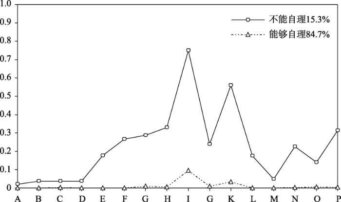
实例数据来自中国人民大学2010~2011执行的北京市城镇老年人(60~95岁)焦虑症状调查, 有效样本量129210(10参见中国国家调查数据库:http://www.cnsda.org/index.php?r=projects/view&id=60493698。感兴趣的读者可以自行下载数据尝试根据附表相应代码进行分析。)。本例中使用了其中的简版老年抑郁量表(GDS-15)总分(gds)、生活自理状况共16个题项(C2A-C2Q), 选项编码为:1. 不费力; 2. 有些困难; 3. 做不了)、年龄(连续变量)、“觉得自己现在老吗” (二分变量, ifold)等题目。
下面通过这个实例简单的介绍通过Mplus软件如何执行上述各变量类型和方法。这里我们对生活自理状况量表进行潜类别分析, 然后依次加入预测变量和结果变量。
(1)潜类别分析
附表1 潜类分析Mplus语句
| Title: Lantent Class Analysis Data: File is older_survey.dat ; Variable: Names = C2A C2B C2C C2D C2E C2F C2G C2H C2I C2J C2K C2L C2M C2N C2P C2Q ifold age gds agesq11(11 年龄平方项(/100)); USEVARIABLES = C2A-C2Q; MISSING are all (-9999) ; CATEGORICAL = C2A-C2Q; CLASSES = C (2); Analysis: TYPE = MIXTURE; Starts = 50 3; PROCESSORS = 4; !根据电脑情况指定 PLOT: TYPE = PLOT3; SERIES = C2A-C2Q (*); Savedata: file is older_survey.txt ; save is cprob; output: tech11 tech14; |
图7
(2)加入预测变量的回归混合模型
在保留的两个类别模型基础上加入连续预测变量(年龄), 预测潜类别变量, 采用R3STEP法, 相应的Mplus语句见网络版附表2。
附表2 加入预测变量回归混合模型的Mplus语句
| Title: Regression Mixture Modeling with Predictive Variable Data: File is older_survey.dat ; Variable: Names = C2A C2B C2C C2D C2E C2F C2G C2H C2I C2J C2K C2L C2M C2N C2P C2Q ifold age gdsagesq; USEVARIABLES = C2A-C2Q; MISSING are all (-9999) ; CATEGORICAL = C2A-C2Q; CLASSES = C (2); AUXILIARY = age (R3STEP);!选择稳健三步法 Analysis: TYPE = MIXTURE; PROCESSORS = 4; PLOT:TYPE = PLOT3; SERIES = C2A-C2Q (*); Savedata: file is older_survey.txt ; save is cprob; output: tech11 tech14; |
如前所述, 因变量为分类潜变量, 这里的回归方程为多项式logistic回归。软件默认第2个类别组为参照组(reference group)。结果表明(见网络版附表3)年龄对第一个类别的回归系数为0.153, SE = 0.014, p < 0.001,说明年龄有助于预测老人所属的类别组。相对于第二类别组(可以自理组), 年龄每大一岁属于第一类别组(不能自理组)的发生比要高16.5%。
附表3 加入预测变量回归混合模型输出结果(部分)
| TESTS OF CATEGORICAL LATENT VARIABLE MULTINOMIAL LOGISTIC REGRESSIONS USING THE 3-STEP PROCEDURE Two-Tailed Estimate S.E. Est./S.E. P-Value C#1 ON AGE 0.153 0.014 11.219 0.000 Intercepts C#1 -12.935 1.031 -12.541 0.000 |
(3)加入分类结果变量的回归混合模型
同样地, 在保留两个类别模型基础上加入自我感觉“是否老了”作为结果变量。该变量有2个选项, 所以采用DCAT法, 语句见网络版附表4。
附表4 加入分类结果变量回归混合模型的Mplus语句
| Title: Regression Mixture Modeling with categorical outcome variable Data: File is older_survey.dat ; Variable: Names = C2A C2B C2C C2D C2E C2F C2G C2H C2I C2J C2K C2L C2M C2N C2P C2Q ifold age gdsagesq; USEVARIABLES = C2A-C2Q; MISSING are all (-9999) ; CATEGORICAL = C2A-C2Q; CLASSES = C (2); AUXILIARY = ifold (DCAT);!选择DCAT法 Analysis: TYPE = MIXTURE; PROCESSORS = 4; LRTSTARTS = 2 1 80 16; PLOT: TYPE = PLOT3; SERIES = C2A-C2Q (*); Savedata: file is older_survey.txt ; save is cprob; output: tech11 tech14; |
分析结果表明(见网络版附表5), 相比于生活自理类别组, 生活不能自理类别的老人其“老人身份认同”的程度要高。具体结果是, 生活不自理类别组选择“觉得自己老了”的概率是0.735, “觉得自己未老”的概率是0.265; 而生活能自理组对应的选择是0.435和0.565。
附表5 加入分类结果变量回归混合模型输出结果(部分)
| EQUALITY TESTS OF MEANS/PROBABILITIES ACROSS CLASSES IFOLD Prob S.E. Odds Ratio S.E. 2.5% C.I. 97.5% C.I. Class 1 Category 1 0.265 0.033 1.000 0.000 1.000 1.000 Category 2 0.735 0.0337 2.133 0.389 1.492 3.049 Class 2 Category 1 0.435 0.016 1.000 0.000 1.000 1.000 Category 2 0.565 0.016 1.000 0.000 1.000 1.000 |
(4)加入连续结果变量的回归混合模型
附表6 加入连续结果变量回归混合模型的Mplus语句
| Title: Regression Mixture Modeling with continuous outcome variable Data: File is older_survey.dat ; Variable: Names = C2A C2B C2C C2D C2E C2F C2G C2H C2I C2J C2K C2L C2M C2N C2P C2Q ifold age gdsagesq; USEVARIABLES = C2A-C2Q; MISSING are all (-9999); CATEGORICAL = C2A-C2Q; CLASSES = C (2); AUXILIARY = gds (BCH);!选择BCH法 Analysis: TYPE = MIXTURE; PROCESSORS = 4; LRTSTARTS = 2 1 80 16; !配合tech14 PLOT: TYPE = PLOT3; SERIES = C2A-C2Q (*); Savedata: file is older_survey.txt ; save is cprob; output: tech11 tech14; |
附表7 加入连续结过变量回归混合模型输出结果(部分)
| EQUALITY TESTS OF MEANS ACROSS CLASSES USING THE BCH PROCEDURE WITH 1 DEGREE (S) OF FREEDOM FOR THE OVERALL TEST GDS Mean S.E. Class 1 4.540 0.211 Class 2 2.903 0.075 Chi-Square P-Value Overall test 52.233 0.000 |
4 小结与展望
总的来说, 回归混合模型目前可以分为两大类别:带有协变量的潜在类别模型和混合结构方程模型。本文主要讨论的带有协变量的潜在类别模型的最新研究方法和软件实现。针对带有协变量的潜在类别模型又可以分成两种不同的类型:包含预测变量和结果变量的模型。就目前的方法学研究来看, 当结果变量是分类变量时, LTB法是最佳选择; 当结果变量是连续变量时BCH和稳健三步法是最佳选择。针对协变量是预测变量的潜在类别模型时, 稳健三步法是最佳选择。
混合模型作为潜变量建模的发展趋势之一, 到目前为止仍处在发展的初期, 很多方法都在探索阶段。尽管已有少数应用研究发表, 但总体来说目前应用研究尚不多。同样地, 回归混合模型作为混合模型的一个分支目前也还是个开放的研究领域, 多数方法是最近3~5年提出的, 而且更新的速度非常快。尽管本文介绍的都是最新的方法, 然而需要注意的是, 在处理不同协变量时所推荐的方法都是小规模模拟研究的结果, 尚需更多模拟研究验证拓展。
另外, 这些方法在处理实际问题时可能存在一些问题, 比如同时存在预测变量和结果变量的情景。在实践中这种情景还是非常普遍的, 但目前尚未有合适的方法。尽管如此, 回归混合模型作为新的方法为我们分析传统问题提供了新的视角。
参考文献
潜在类别分析技术在心理学研究中的应用
潜在类别分析是通过对类别型的外显变量和潜在变量之间的关系建立统计模型,根据模型参数得到各种潜在类别的具体外在表现的潜在特征分类技术。该分析方法主要应用于心理行为特征的分类、控制认知心理实验中被试个体差异引起的系统误差、评价临床心理诊断的精确性,以及心理测验中的项目分析、信度分析、结构分析等。对此方法的优劣进行分析比较,表明:该方法可以与其他测量理论相结合进一步拓展其在心理测量中的应用,也可在纵向数据和多水平数据中应用。在应用中亦有提升方法技术的空间。
Auxiliary variables in mixture modeling: Three-step approaches using M plus
DOI:10.1080/10705511.2014.915181
URL
[本文引用: 5]

This article discusses alternatives to single-step mixture modeling. A 3-step method for latent class predictor variables is studied in several different settings, including latent class analysis, latent transition analysis, and growth mixture modeling. It is explored under violations of its assumptions such as with direct effects from predictors to latent class indicators. The 3-step method is also considered for distal variables. The Lanza, Tan, and Bray (2013) method for distal variables is studied under several conditions including violations of its assumptions. Standard errors are also developed for the Lanza method because these were not given in Lanza et al. (2013).
Auxiliary Variables in Mixture Modeling: Using the BCH Method in Mplus to Estimate a Distal Outcome Model and an Arbitrary Secondary Model
.
Relating latent class membership to continuous distal outcomes: Improving the LTB approach and a modified three-step implementation
DOI:10.1080/10705511.2015.1049698
URL
[本文引用: 7]
Latent class analysis often aims to relate the classes to continuous external consequences (“distal outcomes”), but estimating such relationships necessitates distributional assumptions. Lanza, Tan, and Bray (2013) suggested circumventing such assumptions with their LTB approach: Linear logistic regression of latent class membership on each distal outcome is first used, after which this estimated relationship is reversed using Bayes’ rule. However, the LTB approach currently has 3 drawbacks, which we address in this article. First, LTB interchanges the assumption of normality for one of homoskedasticity, or, equivalently, of linearity of the logistic regression, leading to bias. Fortunately, we show introducing higher order terms prevents this bias. Second, we improve coverage rates by replacing approximate standard errors with resampling methods. Finally, we introduce a bias-corrected 3-step version of LTB as a practical alternative to standard LTB. The improved LTB methods are validated by a simulation study, and an example application demonstrates their usefulness.
Estimating the association between latent class membership and external variables using bias-adjusted three-step approaches
Robustness of stepwise latent class modeling with continuous distal outcomes
DOI:10.1080/10705511.2014.955104
URL
Recently, several bias-adjusted stepwise approaches to latent class modeling with continuous distal outcomes have been proposed in the literature and implemented in generally available software for latent class analysis. In this article, we investigate the robustness of these methods to violations of underlying model assumptions by means of a simulation study. Although each of the 4 investigated methods yields unbiased estimates of the class-specific means of distal outcomes when the underlying assumptions hold, 3 of the methods could fail to different degrees when assumptions are violated. Based on our study, we provide recommendations on which method to use under what circumstances. The differences between the various stepwise latent class approaches are illustrated by means of a real data application on outcomes related to recidivism for clusters of juvenile offenders.
Distributional assumptions of growth mixture models: Implications for overextraction of latent trajectory classes
DOI:10.1037/1082-989X.8.3.338
URL
PMID:14596495
[本文引用: 2]
Abstract Growth mixture models are often used to determine if subgroups exist within the population that follow qualitatively distinct developmental trajectories. However, statistical theory developed for finite normal mixture models suggests that latent trajectory classes can be estimated even in the absence of population heterogeneity if the distribution of the repeated measures is nonnormal. By drawing on this theory, this article demonstrates that multiple trajectory classes can be estimated and appear optimal for nonnormal data even when only 1 group exists in the population. Further, the within-class parameter estimates obtained from these models are largely uninterpretable. Significant predictive relationships may be obscured or spurious relationships identified. The implications of these results for applied research are highlighted, and future directions for quantitative developments are suggested.
Estimating latent structure models with categorical variables: One-step versus three-step estimators
DOI:10.1093/pan/mph001
URL
[本文引用: 3]
We study the properties of a three-step approach to estimating the parameters of a latent structure model for categorical data and propose a simple correction for a common source of bias. Such models have a measurement part (essentially the latent class model) and a structural (causal) part (essentially a system of logit equations). In the three-step approach, a stand-alone measurement model is first defined and its parameters are estimated. Individual predicted scores on the latent variables are then computed from the parameter estimates of the measurement model and the individual observed scoring patterns on the indicators. Finally, these predicted scores are used in the causal part and treated as observed variables. We show that such a naive use of predicted latent scores cannot be recommended since it leads to a systematic underestimation of the strength of the association among the variables in the structural part of the models. However, a simple correction procedure can eliminate this systematic bias. This approach is illustrated on simulated and real data. A method that uses multiple imputation to account for the fact that the predicted latent variables are random variables can produce standard errors for the parameters in the structural part of the model.
Relating latent class analysis results to variables not included in the analysis
Retrieved from
Latent class and latent transition analysis: With applications in the social, behavioral, and health sciences
.
Latent class analysis with distal outcomes: A flexible model-based approach
DOI:10.1080/10705511.2013.742377
URL
PMID:4240499
[本文引用: 2]
Although prediction of class membership from observed variables in latent class analysis is well understood, predicting an observed distal outcome from latent class membership is more complicated. A flexible model-based approach is proposed to empirically derive and summarize the class-dependent density functions of distal outcomes with categorical, continuous, or count distributions. A Monte Carlo simulation study is conducted to compare the performance of the new technique to 2 commonly used classify-analyze techniques: maximum-probability assignment and multiple pseudoclass draws. Simulation results show that the model-based approach produces substantially less biased estimates of the effect compared to either classify-analyze technique, particularly when the association between the latent class variable and the distal outcome is strong. In addition, we show that only the model-based approach is consistent. The approach is demonstrated empirically: latent classes of adolescent depression are used to predict smoking, grades, and delinquency. SAS syntax for implementing this approach using PROC LCA and a corresponding macro are provided.
A multifoci person-centered perspective on workplace affective commitment: A latent profile/factor mixture analysis
DOI:10.1177/1094428109356476
URL
[本文引用: 1]
ABSTRACT The current study aims to explore the usefulness of a person-centered perspective to the study of workplace affective commitment (WAC). Five distinct profiles of employees were hypothesized based on their levels of WAC directed toward seven foci (organization, workgroup, supervisor, customers, job, work, and career). This study applied latent profile analyses and factor mixture analyses to a sample of 404 Canadian workers. The construct validity of the extracted latent profiles was verified by their associations with multiple predictors (gender, age, tenure, social relationships at work, workplace satisfaction, and organizational justice perceptions) and outcomes (in-role performance, organizational citizenship behaviors, and intent to quit). The analyses confirmed that a model with five latent profiles adequately represented the data: (a) highly committed toward all foci; (b) weakly committed toward all foci; (c) committed to their supervisor and moderately committed to the other foci; and (d) committed to their career and moderately uncommitted to the other foci; (e) committed mostly to their proximal work environment. These latent profiles present theoretically coherent patterns of associations with the predictors and outcomes, which suggests their adequate construct validity. [ABSTRACT FROM AUTHOR] Copyright of Organizational Research Methods is the property of Sage Publications Inc. and its content may not be copied or emailed to multiple sites or posted to a listserv without the copyright holder's express written permission. However, users may print, download, or email articles for individual use. This abstract may be abridged. No warranty is given about the accuracy of the copy. Users should refer to the original published version of the material for the full abstract. (Copyright applies to all Abstracts.)
Understanding linkages among mixture models
DOI:10.1080/00273171.2013.827564
URL
PMID:26745595
[本文引用: 1]
The methodological literature on mixture modeling has rapidly expanded in the past 15 years, and mixture models are increasingly applied in practice. Nonetheless, this literature has historically been diffuse, with different notations, motivations, and parameterizations making mixture models appear disconnected. This pedagogical review facilitates an integrative understanding of mixture models. First, 5 prototypic mixture models are presented in a unified format with incremental complexity while highlighting their mutual reliance on familiar probability laws, common assumptions, and shared aspects of interpretation. Second, 2 recent extensionshybrid mixtures and parallel-process mixturesare discussed. Both relax a key assumption of classic mixture models but do so in different ways. Similarities in construction and interpretation among hybrid mixtures and among parallel-process mixtures are emphasized. Third, the combination of both extensions is motivated and illustrated by means of an example on oppositional defiant and depressive symptoms. By clarifying how existing mixture models relate and can be combined, this article bridges past and current developments and provides a foundation for understanding new developments.
Latent class modeling with covariates: Two improved three-step approaches
DOI:10.1093/pan/mpq025
URL
[本文引用: 5]
Researchers using latent class (LC) analysis often proceed using the following three steps: (1) an LC model is built for a set of response variables, (2) subjects are assigned to LCs based on their posterior class membership probabilities, and (3) the association between the assigned class membership and external variables is investigated using simple cross-tabulations or multinomial logistic regression analysis. Bolck, Croon, and Hagenaars (2004) demonstrated that such a three-step approach underestimates the associations between covariates and class membership. They proposed resolving this problem by means of a specific correction method that involves modifying the third step. In this article, I extend the correction method of Bolck, Croon, and Hagenaars by showing that it involves maximizing a weighted log-likelihood function for clustered data. This conceptualization makes it possible to apply the method not only with categorical but also with continuous explanatory variables, to obtain correct tests using complex sampling variance estimation methods, and to implement it in standard software for logistic regression analysis. In addition, a new maximum likelihood (ML)u2014based correction method is proposed, which is more direct in the sense that it does not require analyzing weighted data. This new three-step ML method can be easily implemented in software for LC analysis. The reported simulation study shows that both correction methods perform very well in the sense that their parameter estimates and their SEs can be trusted, except for situations with very poorly separated classes. The main advantage of the ML method compared with the Bolck, Croon, and Hagenaars approach is that it is much more efficient and almost as efficient as one-step ML estimation.
Residual diagnostics for growth mixture models: Examining the impact of a preventive intervention on multiple trajectories of aggressive behavior
DOI:10.1198/016214505000000501
URL
[本文引用: 1]
Growth mixture modeling has become a prominent tool for studying the heterogeneity of developmental trajectories within a population. In this article we develop graphical diagnostics to detect misspecification in growth mixture models regarding the number of growth classes, growth trajectory means, and covariance structures. For each model misspecification, we propose a different type of empirical Bayes residual to quantify the departure. Our procedure begins by imputing multiple independent sets of growth classes for the sample. Then, from these so-called "pseudoclass" draws, we form diagnostic plots to examine the averaged empirical distributions of residuals in each such class. Our proposals draw on the property that each single set of pseudoclass adjusted residuals is asymptotically normal with known mean and (co)variance when the underlying model is correct. These methods are justified in simulation studies involving two classes of linear growth curves that also differ by their covariance structures. These are then applied to longitudinal data from a randomized field trial that tests whether children's trajectories of aggressive behavior could be modified during elementary and middle school. Our diagnostics lead to a solution involving a mixture of three growth classes. When comparing the diagnostics obtained from multiple pseudoclasses with those from multiple imputations, we show the computational advantage of the former and obtain a criterion for determining the minimum number of pseudoclass draws.
