

1 引言
在心理学、行为学和其他社会科学研究领域, 研究者经常要通过潜变量(Latent Variables, LVs), 即不能直接观测的变量, 来研究如智力、人格、态度、能力等抽象的构念(Construct)、特质(Trait)或因子(Factor)。一个潜变量往往对应着若干个相关的、可直接观测的外显变量(Manifest Variables)。潜变量可以看作其对应外显变量的抽象和概括, 而外显变量则可视为特定潜变量的反映指标。结构方程模型(Structural Equation Modeling, SEM)是公认的用于分析潜变量间关系最强有力的现代统计方法, 是心理学、教育学和行为学等领域最常用的分析方法之一(侯杰泰, 温忠麟, 成子娟, 张雷, 2004; Lee & Song, 2012; 王孟成, 2014)。SEM流行的一个重要原因在于其灵活性, 包括验证性因子分析模型、中介模型和潜变量增长曲线模型在内的许多模型都能以SEM的形式表征出来。
传统的SEM包括测量模型和结构模型两个部分, 其中测量模型将外显变量与对应的潜变量关联起来, 通常是一个验证性因子分析(Confirmatory Factor Analysis, CFA)模型, 主要用于检验潜变量的因子结构。其定义如下:
其中${{y}_{i}}$(p×1)为第i个被试在p个相关的外显变量上的观测值, μ (p×1)为截距项, Λ (p×q)为因子载荷矩阵, 用于反映外显变量yi和潜变量ωi (q×1)之间的关系, εi (p×1)是外显变量的测量误差项, 服从于N[0,Ψε]的分布。模型包含以下假设:测量误差和潜变量间不存在相关; 测量误差的方差协方差矩阵Ψε为对角矩阵, 即测量误差间不存在相关。传统的测量模型还通常假设潜变量的数目以及潜变量与外显变量间的关系已知, 且每个外显变量只负载在一个潜变量上, 不存在交叉载荷。
结构模型主要用于分析潜变量之间的“因果效应”, 其定义如下:令ωi = (ηiT, ξiT )T, 其中ηi (q1×1)是外源潜变量(Exogenous LVs), ${{\xi }_{i}}$(q2×1)是内生潜变量(Endogenous LVs),
其中Λω = (Π, Γ)、Π(q1×q1)和Γ(q1×q2)是路径系数矩阵, Π反映了内生潜变量之间的效应, 而Γ则反映了外源潜变量对内生潜变量的效应。ξi服从于N[0,Φξ]的分布, δi (q1×1)为残差项, 服从于N[0,Ψδ]的分布。
结构方程模型的分析步骤通常包括模型设定与识别、模型拟合评估、模型修正和参数估计。与传统的路径分析方法相比, 结构方程模型考虑了外显变量的测量误差, 对潜变量间关系的估计更加准确(李锡钦, 2011)。
2 贝叶斯结构方程模型
结构方程模型的主要估计方法包括频率学派方法(如, 极大似然估计)和贝叶斯方法两类。尽管目前对频率学派方法的应用更多, 但近年来, 由于贝叶斯方法的流行及其在统计建模中的诸多优势, 关于贝叶斯结构方程模型的方法类和应用类研究数量稳步增长。尤其是自2012年以来, 贝叶斯结构方程模型的应用研究数量大幅增加(van de Schoot, Winter, Ryan, Zondervan-Zwijnenburg, & Depaoli, 2017)。
贝叶斯方法和频率学派方法本质的区别是:频率学派将未知参数看作常数, 根据样本参数估计总体参数; 而贝叶斯方法则将未知参数视为随机变量, 分析的目的是得到未知参数的后验分布(王孟成, 邓倩文, 毕向阳, 2017)。在用贝叶斯方法分析SEM时, 研究者可以根据理论或以往研究结果确定未知参数或潜变量的先验分布, 如果没有准确的先验信息也可以提供无信息先验分布(如, 均匀分布)或模糊信息先验分布(如, 方差极大的正态分布); 根据贝叶斯公式, 结合先验分布和数据似然函数可以得到未知参数和潜变量的后验分布; 再采用马尔科夫链蒙特卡罗(Markov Chain Monte Carlo, MCMC)算法(如, Gibbs抽样法和Metropolis-Hastings算法等)从后验分布中迭代地抽取大量样本; 通过抽取的样本估计后验分布的均值、可信区间(Credible Interval)及其它统计量, 进而进行统计推断(李锡钦, 2011)。
采用贝叶斯方法分析SEM的具体步骤包括:
(1)设定模型并为未知参数提供先验信息:令k = 1, …, p, h = 1, …, q1, 对于SEM中不同的未知参数提供如下所示的共轭先验分布(李锡钦, 2011):
其中ΛkT是载荷矩阵Λ的第k行, ΛTωh是路径系数矩阵Λω的第h行, μ0, Λ0k, Λ0ωh, ρ0和正定矩阵R0, Hμ0, H0k, H0ωh是根据理论或以往研究结果给定的超参数值, 反映先验信息及研究者对先验信息准确性的把握;
(2)设定MCMC算法迭代次数, 在其收敛后进行模型拟合评估和参数估计。算法是否达到收敛可以通过踪迹图和潜在尺度缩减因子进行评估(详见王孟成 等, 2017);
(3)模型与数据的整体拟合程度可以通过后验预测检验(Posterior Predictive Checking)评估;
(4)为避免先验信息主观性的影响, 研究者可以通过敏感性分析(Sensitivity Analysis; Greenland, 2001)检验不同先验信息下估计结果是否稳定, 增强结果的可靠性。
与传统方法相比, 贝叶斯结构方程模型有着诸多优势, 例如:(1)相比于频率学派的方法, 基于抽样的贝叶斯方法较少地依赖大样本渐近理论, 因此在小样本中依旧表现优良(Muthén & Asparouhov, 2012); (2)贝叶斯结构方程模型的分析基于原始观测值, 这相比于传统方法关注的协方差矩阵更易于处理。因此更易于处理复杂的模型和数据情况, 如存在缺失值的数据、潜变量间存在非线性关系的情况等, 而传统方法在这种情况下容易遇到模型识别问题(李锡钦, 2011); (3)在模型拟合评估、模型比较和参数估计方面, 贝叶斯方法能够提供更有效的统计量(Pan, Ip, & Dubé, 2017); (4)贝叶斯方法能够灵活地在模型估计中纳入先验信息, 如预实验和前人研究结果, 而有效的先验信息可以使未知参数估计更加准确(Yuan & MacKinnon, 2009; Zhang, Hamagami, Wang, & Nesselroade, 2007)。
尽管采用贝叶斯结构方程模型有着诸多优点, 能够更好地满足应用研究者在实证研究中的需求, 如处理复杂模型、小样本问题等情况, 但其在国内心理学领域的应用不足。本文将介绍几类常用的贝叶斯结构方程模型及其应用研究进展, 包括验证性因子分析、结构方程模型、中介模型、潜变量增长曲线模型、多组模型和多层模型, 旨在为应用研究者介绍新的研究工具, 促进其在国内心理学研究中的应用。
3 分类
3.1 经典贝叶斯结构方程模型
3.1.1 贝叶斯验证性因子分析
验证性因子分析常被用于根据理论假设去验证外显变量和潜变量间的关系。在传统的CFA模型中, 局部独立性(Local Independence)假设要求给定了潜变量的值后, 外显变量之间不再存在相关, 即测量误差项的方差协方差矩阵Ψε中非对角线元素的值均被限制为0。此外, 传统的CFA模型一般不允许存在交叉载荷。但是在实际研究中, 这种严格的约束条件容易导致模型拟合不好甚至被拒绝(Muthén & Asparouhov, 2012)。一些研究者指出, 传统方法对模型施加的限制是过于严格的、甚至是不必要的, 这种限制在大样本情况下很容易拒绝实际上和数据拟合良好的模型(Lu, Chow, & Loken, 2016; Marsh et al., 2009; Muthén & Asparouhov, 2012)。且有研究者发现, 在实际数据分析中对模型添加过多的约束条件还会导致未知参数估计的准确性降低(Asparouhov & Muthén, 2009; Hsu, Troncoso Skidmore, Li, & Thompson, 2014)。
在传统方法中, 为了解决这种限制带来的问题, 研究者往往会结合理论和修正指数(Modification Index; Sörbom, 1989)的建议, 在模型中增加交叉载荷或测量误差间的相关。但是这种基于修正指数的方法仍然存在一些局限, 例如: (1)由于需要逐个参数进行修正, 当需要修正的参数较多时, 修正的过程耗时、繁琐; (2)容易导致模型的过拟合, 削弱其泛化能力(Maccallum, Roznowski, & Necowitz, 1992); (3)难以找到全局最优的模型(Chou & Bentler, 1990); (4)容易导致一类错误率增大(Draper, 1995)等。
Muthén和Asparouhov (2012)创新地提出了一种结合了探索和验证方法的贝叶斯验证性因子分析模型, 放宽了模型对于测量误差相关或交叉载荷的限制。在传统方法中, 交叉载荷和测量误差间的相关被严格限制为0, 这既是基于模型简洁性的考虑, 也是因为如果自由估计这些参数容易导致模型不可识别。但是Muthén和Asparouhov (2012)提出的方法在保证模型可识别的同时, 可以通过对交叉载荷提供一个均值为0、方差极小的正态先验分布, 或对误差项矩阵提供合适的逆Wishart分布来放宽对其的限制。模拟研究显示, 该方法在放宽对于交叉载荷或测量误差相关的限制时, 得到的显著的交叉载荷或测量误差相关的数目比修正指数方法得到的更少, 且模型拟合在一次分析中就可以得到满意的结果, 而传统方法通常需要进行多次修正。
但是Muthén和Asparouhov (2012)提出的这种方法在放宽模型限制的同时, 也容易导致较多非零交叉载荷或测量误差相关的产生(Lu, Chow, & Loken, 2016), 使得因子载荷矩阵或误差项矩阵过于复杂。因而模型容易出现过拟合的情况, 对研究结果的解释和重复造成困难。
Lu等人(2016)指出Muthén和Asparouhov (2012)的方法本质上是将贝叶斯Ridge正则化(Regularization)方法应用于CFA模型中。针对其存在的上述问题, Lu等人(2016)引入了另一种贝叶斯正则化方法:通过对载荷矩阵提供spike-and- slab先验分布, 保留重要的交叉载荷, 将其它微弱的交叉载荷压缩到零。这种方法避免了Ridge正则化方法可能导致的模型过拟合, 及其对重要交叉载荷的过度压缩等问题。
Pan等人(2017)则针对误差项的方差协方差矩阵, 将协方差Lasso (Least absolute shrinkage and selection operator)正则化方法引入CFA模型。通过估计稀疏化的误差协方差矩阵, 在放宽对测量误差相关限制的同时, 将微弱的、不重要的测量误差相关向零压缩, 避免因为测量误差相关过多而导致的模型过拟合或误差项矩阵不正定等问题。其实证研究发现在允许“少量”测量误差相关的情况下, CFA模型的简约性和拟合程度都得到了满足。
自放宽模型限制的思想被提出以来, 由于其诸多优点, 采用贝叶斯CFA进行数据分析的应用研究越来越多。基于贝叶斯方法在处理复杂模型时的优良特性, Golay, Reverte, Rossier, Favez和Lecerf (2013)重新分析了韦氏智力量表的四因子结构, 分别检验了二阶因子模型和双因子(Bifactor)模型, 结果显示贝叶斯方法在模型识别和估计上都比极大似然估计表现得更好; 而Falkenström, Hatcher和Holmqvist (2015)在检验病人版工作智力量表的结构效度时发现, 极大似然估计显示模型拟合较差, 但采用贝叶斯方法放宽对测量误差相关的限制后, 模型和数据拟合很好; 此外, 由于小样本中贝叶斯方法对于参数的估计更加准确(Muthén & Asparouhov, 2012), Crenshaw, Christensen, Baucom, Epstein和Baucom (2016)在临床的小样本研究中使用贝叶斯CFA方法修订了沟通模式量表(52名被试, 模型有18个未知参数,
包括9个因子载荷和9个测量误差方差); 而由于与传统的极大似然估计方法相比, 贝叶斯方法在小样本的情况下对因子分的估计更加准确(Muthén & Asparouhov, 2012),Alessandri和de Pascalis (2017)在脑电实验研究中采用贝叶斯CFA估计51名被试“生活导向”因子的因子分, 再用于后续因子间关系的分析中。
3.1.2 贝叶斯结构方程模型
在测量模型的基础上, 结构模型被用于检验不受测量误差影响的潜变量间的“因果效应”。正如本文第二部分所述, 在采用贝叶斯方法估计结构方程模型时, 可以通过对未知参数和潜变量提供合适的先验分布, 结合数据得到其后验分布, 进而进行统计推断。
随着对测量模型限制的放宽, 对结构模型中未知参数的估计也更加准确。Pan等人(2017)在建立测量模型时采用贝叶斯Lasso方法对误差协方差矩阵进行估计, 结果发现:与传统方法相比, 贝叶斯Lasso方法下对结构模型中路径系数的估计偏差也更小。
此外, 在对结构模型的估计中, 使用贝叶斯方法可以对所有的路径系数提供一定的先验分布。和贝叶斯验证性因子分析相似的是, Muthén和Asparouhov (2012)指出可以对原先被限定为0的路径系数提供均值为0, 方差极小的正态先验分布来放宽对其的限制, 在一次估计中可以同时实现对模型探索和验证。
为了方便研究者应用这种方法, 我们将以Muthén和Asparouhov (2012)建立的贝叶斯结构方程模型为例, 详细介绍在测量模型和结构模型中同时使用信息先验的具体实现步骤。该研究重新分析了Kaplan (2009)的追踪研究, 研究收集了6677名公立学校十年级学生的数据, 所建立的模型如图1所示。模型包含以下假设:学生六年级的科学成绩和家庭社会经济地位通过影响其十年级的科学成绩进而影响学生的科学成就; 而教师的科学认证水平通过影响学生的参与程度, 进而影响学生对课程挑战性的感知程度, 最终通过学生十年级的科学成绩影响其科学成就。
图1
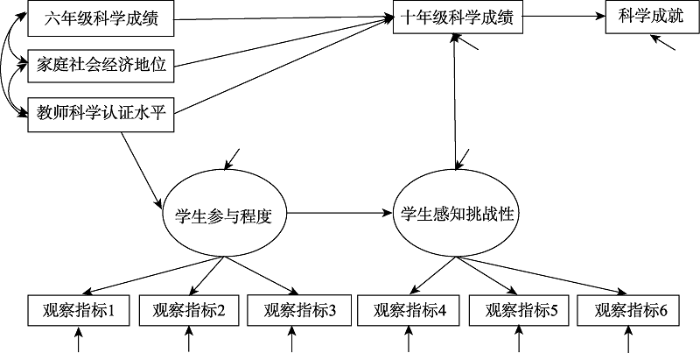
图1
科学成就的结构方程模型图(改编自Kaplan(2009))
研究者采用传统的极大似然估计发现, 模型拟合较差, 假设模型被拒绝(RMSEA = 0.081, CFI = 0.844), 修正指数显示模型中存在大量需要被修正的参数。而无信息先验下贝叶斯方法的估计结果与之相似, 后验预测检验区间不包括零, 模型拟合较差(95% CI [1644, 1720])。
基于前文中放宽模型限制的思想, 在对数据进行标准化处理后, Muthén和Asparouhov (2012)针对结构模型中原先被固定为0的11个参数提供了均值0, 方差为0.01的正态分布先验, 即允许这些参数有95%的变异落在(-0.2, 0.2)之间。由于已经对数据进行了标准化处理, 上述设定的先验分布理论上能较好地覆盖那些可能被忽略的效应的范围。研究者针对六年级科学成绩、家庭社会经济地位和教师科学认证水平三个变量指向6个观察指标的18个路径系数也提供了同样的先验分布, 在传统方法中, 这些路径系数如果被自由估计将意味着6个观察指标存在项目功能差异。但是在这里, 研究者仅仅通过提供均值为0, 方差极小的先验分布来放宽对其严格的限制。
此外, 研究者还放宽了对于6个观察指标的交叉载荷及测量误差相关的限制。其中, 对交叉载荷同样提供了均值为0, 方差为0.01的正态先验分布, 而对误差项矩阵提供IW (I, 30)的逆Wishart分布。模型对应的Mplus代码详见Muthén和Asparouhov (2012)的补充材料。
结果发现与未放宽模型限制的模型相比, 模型拟合得到了提升, 后验预测检验区间包括0 (95% CI [-24, 44]), 后验预测p值为0.276。同时还额外发现了6个显著的结构模型参数, 及11对显著的测量误差相关, 但其估计值均较小1(1 研究者将显著的测量误差相关仅视为冗余参数(nuisance parameters)。)。Muthén和Asparouhov (2012)在文章中指出, 如果使用传统的极大似然估计, 上述放宽限制后的模型将是不可识别的, 但在贝叶斯框架下可以避免这种情况。同时他们还指出在放宽模型的限制后, 模型的收敛率降低, 需要更多的迭代次数和更长的运算时间才能得到模型估计结果。关于上述内容的讨论, 感兴趣的读者可参考Muthén和Asparouhov (2012), 本文不再赘述。
此外, 在实证研究中, 越来越多的应用研究者也开始采用这种方法。Scherer, Siddiq和Teo (2015)基于所研究的潜变量间存在概念重叠的情况, 认为建模时必须要考虑交叉载荷, 但传统方法中加入过多的交叉载荷会出现模型识别或估计问题。基于贝叶斯结构方程模型的思想, Scherer等人(2015)采用了贝叶斯方法放宽对测量模型的限制, 并在此基础上建立结构模型以检验教师对信息技术的利用与教师自身特征的关系。Salarzadeh, Moghavvemi, Wan, Babashamsi和Arashi (2017)同样采用该方法研究了影响学生使用电子学习平台意愿的因素, 并对比极大似然估计和贝叶斯估计的结果, 发现贝叶斯估计下模型估计结果更准确, 误差均方根和绝对平均误差更小。
3.1.3 贝叶斯中介模型
中介分析在心理学领域中扮演着非常重要的角色, 它可以用于解释自变量对因变量的作用机制, 有助于已有理论的验证和新的理论的构建(罗胜强, 姜嬿, 2014)。在检验中介效应时, 关键是检验间接效应的显著性, 即自变量是否会通过中介变量“显著地”影响因变量。在Yuan和MacKinnon (2009)的贝叶斯中介建模方法出现之前, 心理学研究中大多数中介效应分析都在频率学派的框架下进行(Nuijten, Wetzels, Matzke, Dolan, & Wagenmakers, 2015)。目前频率学派中检验间接效应显著性的常用方法是Sobel法和Bootstrap法。其中, Sobel法即直接检验直接效应系数乘积的显著性(H0: ab = 0; a, b即两个直接效应系数), 但是该方法需要假设系数的乘积服从正态分布, 否则估计将产生偏差。而这个假设在实际数据分析中往往很难被满足, 但Bootstrap法通过构建区间估计可以避免这一问题(温忠麟, 叶宝娟, 2014)。
在贝叶斯框架下的中介分析则是通过MCMC法进行, 这种方法基于从后验分布中抽取的样本进行参数估计。在获取了直接效应系数的后验分布后, 可以很容易地对参数的各种函数形式进行估计, 如两个直接效应系数的乘积, 而且该方法易于构造间接效应的可信区间(Yuan & MacKinnon, 2009)。因此贝叶斯方法易于处理复杂的中介模型, 如贝叶斯序列中介模型(Tofighi & Mackinnon, 2016), 有调节的中介模型(Wang & Preacher, 2015)等。而传统方法在处理复杂模型时则常常会遇到模型识别和估计问题(Kenny, Korchmaros, & Bolger, 2003)。
此外, 贝叶斯中介模型不需要假设系数乘积服从正态分布。以往的研究发现, 除无信息先验条件下贝叶斯方法和传统方法的估计结果比较相似外, 在信息先验和模糊信息先验条件下, 贝叶斯方法的检验力都更高, 对于参数的估计也更加准确(MacKinnon, Lockwood, & Williams, 2004; Tofighi & MacKinnon, 2011; Tofighi & Mackinnon, 2016), 在小样本中表现也更好(Miočević, MacKinnon, & Levy, 2017)。
由于中介分析的重要性及贝叶斯中介模型的优良特性, 采用贝叶斯方法检验中介效应的研究也越来越多。鉴于贝叶斯分析不依赖于参数的正态分布假设, Shuck, Zigarmi和Owen (2015)通过贝叶斯多重中介模型检验了工作投入、员工敬业度、工作热情在基本心理需求对工作意图的影响中的中介效应; 而由于研究的样本量较少, Zeman, Dallaire, Folk和Thrash (2017)同样采用该方法检验了在监禁风险经历和环境风险对儿童精神障碍的影响中儿童情绪管理的中介效应; 此外, 结合贝叶斯中介建模和贝叶斯CFA放宽测量模型限制的方法, Jacobson, Lord和Newman (2017)验证了焦虑通过情绪智力中介影响抑郁症状。
3.2 贝叶斯潜变量增长曲线模型
纵向研究也称追踪研究, 它通过对研究对象进行长期追踪观察、重复测量个体有关变量, 能够观察较为完整的发展过程, 发现发展过程中的一些关键转折。与横断研究相比, 纵向研究设计最大的优点是可以合理地推导变量之间的因果关系, 是心理学研究中一种重要的研究方法(刘红云, 孟庆茂, 2003)。
目前在分析追踪数据的结构方程建模中, 潜变量增长曲线模型(Latent Growth Curve Model, LGCM; Bollen & Curran, 2006)应用非常广泛。该模型不仅能够分析总体平均变化趋势, 还能分析不同个体发展轨迹变化的差异及其如何受到预测变量的影响。
LGCM适用于在几个固定时间点观测得到的纵向研究数据(刘红云, 孟庆茂, 2003)。一个简单的非条件线性潜变量增长曲线模型的定义如下(王济川, 王小倩, 姜宝法, 2011):
其中yti是第i个个体在时间点t的外显变量数据, η0i和η1i是随机系数, 描述了数据随时间变化的特点, 也被称为发展因子(Growth Factors), λt是时间分值, εti是变量在时间点t的复合误差项, 表示随机测量误差和第i个个体的特定时间效应。在(5)式和(6)式中, η0和η1分别反映变量的平均初始水平和变量的平均变化率, 故而η0i和η1i分别被称为潜截距发展因子和潜斜率发展因子, ζ0i和ζ1i表示残差项, 其方差能反映研究对象的个体间变异。
此外, 研究者还可以在模型中纳入一些预测变量来预测上述两个潜发展因子。而如果变量的发展轨迹为非线性, 也可以通过引入时间分值的二阶或高阶函数, 或通过设定自由时间分值等方式来检验非线性的发展轨迹(Meredith & Tisak, 1990)。
在估计潜变量增长曲线模型时, 贝叶斯方法相比于传统估计方法具有许多优势。首先, 追踪数据情况较为复杂, 可能会出现测量时间间隔不相等、发展轨迹非线性、数据不满足正态分布等情况, 因此有时需要进行复杂的数据转换, 而贝叶斯估计依赖于原始观测值而非方差协方差矩阵, 更易于处理这种数据转换的情况(Gelman et al., 2014); 其次, 传统方法在处理复杂的LGCM时容易出现估计问题甚至是模型识别问题, 而贝叶斯方法能够更有效地估计复杂模型(Zhang et al., 2007); 第三, 追踪研究中普遍存在缺失数据(叶素静, 唐文清, 张敏强, 曹魏聪, 2014), 而贝叶斯方法在处理缺失数据时表现更好(李锡钦, 2011); 此外, 贝叶斯方法在小样本情况下表现更好(Gelman, Carlin, Stern, & Rubin, 2003), Zhang等人(2007)发现使用贝叶斯方法甚至可以估计只有20个被试在4个不同时间点测量的潜变量增长曲线模型, 这使得贝叶斯方法具有极高的应用价值。
在实证研究中, Winans-Mitrik等人(2014)指出比起依赖假设检验的传统频率学派方法, 贝叶斯方法能够提供更加稳定的推断, 更符合临床评估的要求, 因而采用贝叶斯LGCM验证失语症干预项目对于语言理解的促进作用, 在对被试的失语症严重程度进行了4次测量后, 发现该干预项目对于失语症有可靠且持续的治疗作用。此外, 由于贝叶斯方法在小样本和数据非正态情况下表现更优良(Gelman et al., 2014), Maier, Bohlmann和Palacios (2016)采用贝叶斯LGCM分析了儿童语言发展中跨语言的联系, 发现英语与西班牙语的词汇表达能力的交互项影响英语词汇表达能力的增长。我们将以这个研究为例, 详细介绍贝叶斯LGCM的建模步骤。
该研究的被试为洛杉矶地区低到中等收入家庭中的177名学龄前儿童, 研究者在秋季学期初、4个月后、6个月后三个时间点对其进行随访。在每次随访中, 通过语言测试及编码员进行行为编码的方式, 测量儿童英语和西班牙语的词汇表达能力与接受能力, 并调查了儿童的人口学变量、教师与班级特征、班级与家庭语言环境等方面的多个协变量。
研究者通过贝叶斯方法处理缺失值, 将缺失观测值作为未知值进行估计。在进行建模分析时, 首先为英语词汇接受能力、英语词汇表达能力、西班牙语词汇接受能力、西班牙语词汇表达能力四个结果变量分别建立非条件潜变量增长曲线模型(图2)。
图2
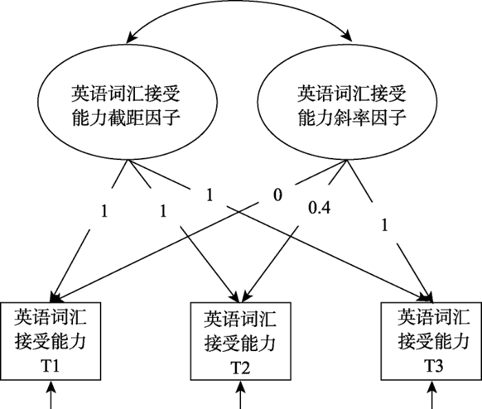
模型为每个变量构造了两个发展因子, 截距与斜率因子的协方差被允许自由估计。每个因子都有对应三个时间点的测量作为它们的观察指标。对于斜率因子, 根据测量的时间间隔, 按照线性关系固定了三次时间点的负载分别为0、0.4、1。而三个时间点中观察指标的残差被允许自由估计。截距和斜率发展因子的均值反映了该变量的总体平均初始值及变化率, 因子的方差则反映了个体间差异。在模型估计时, 研究者采用了Mplus 6.11中的贝叶斯估计并提供默认的无信息先验分布。而在建立了非条件模型之后, 研究者进一步将协变量纳入到模型中以预测截距因子和斜率因子, 建立条件潜变量增长曲线模型。
结果发现被试群体的英语词汇接受能力、英语词汇表达能力、西班牙语词汇接受能力以及西班牙语词汇表达能力对应的4个非条件模型拟合良好, PPp值分别为0.56 (后验预测检验区间95% CI [-13.51, 10.46]), 0.26 (95% CI [-8.38, 16.85]), 0.53 (95% CI [-11.33, 9.66]), 0.48 (95% CI [-12.67, 11.81])。各个斜率因子估计结果均大于0, 表明4种词汇能力均随着时间而逐渐增长。在4种能力上, 不同个体在初始水平和变化率上表现出显著的个体差异(即截距和斜率因子的方差均显著不为0)。
加入协变量后的条件模型的PPp值分别为0.31 (95% CI [-26.96, 52.53]), 0.21 (95% CI [-23.84, 58.95]), 0.29 (95% CI [-32.40, 51.26]), 0.34 (95% CI [-28.35, 52.86]) , 模型拟合结果均为良好。参数估计结果显示, 在4个条件模型中, 年龄对截距因子都有正向预测作用, 表明年龄较大的学龄前儿童倾向于拥有较高的初始词汇量。家庭中的英语接触水平也能够正向预测儿童英语词汇能力, 而对西班牙语的初始词汇能力有负向影响。另外, 由于贝叶斯方法在估计因子得分上的优势, 研究者在贝叶斯LGCM下得到了每个被试在截距因子和斜率因子上的值, 进一步探究了英语和西班牙语词汇能力间的相互联系, 但由于本文篇幅有限, 在此不做赘述。
上述实例简单介绍了贝叶斯方法在潜变量增长曲线模型中的应用。目前, 在大部分采用贝叶斯LGCM的研究中, 研究者仅仅是将模型估计方法改为贝叶斯估计, 对于参数估计往往提供软件默认的无信息先验。未来研究可以考察合适的先验分布对于潜变量增长曲线模型中参数估计的影响, 进一步发挥贝叶斯方法在模型拟合和参数估计中的优势。
3.3 贝叶斯多组结构方程模型
在实证研究中, 研究者常常会根据某些变量将人群分为多个组别, 如根据性别划分出男女两组。在这种情况下, 数据往往表现为组数较少、每组观测值较多且组内观测值均是独立的, 即多组数据。在多组数据的结构方程建模中, 研究者可以通过分组建立模型来研究不同组间模型的相似性和差异性。多组结构方程模型所感兴趣的是检验不同组间模型的各种不变性假设(李锡钦, 2011)。
不变性假设的检验首先需要在测量模型中进行, 即测量不变性(Measurement Invariance)假设。检验测量不变性可以通过一系列嵌套步骤进行, 按顺序包括结构不变性(各组具有相同的因子结构), 即量表条目在不同组中均被负载到相同的潜变量上; 载荷不变性(条目载荷跨组相同); 截距不变性(条目截距跨组相同)以及误差方差/协方差不变性(条目误差方差跨组相同) (Vandenberg & Lance, 2000)。测量不变性是进行潜变量水平参数的跨组比较的基础, 即对结构不变性的检验, 结构不变性包括因子方差/协方差不变性和因子均数结构不变性(王济川 等, 2011)。当模型不符合跨组截距不变性时, 跨组因子分的差异通常不能清楚地反映潜变量水平的真实差异(Schmitt & Kuljanin, 2008)。
在检验不变性时, 传统方法首先需要确定每个组的基线模型; 然后构建组态模型(Configural Model), 即整合各组的基线模型; 在组态模型中对相应参数(如, 载荷、截距)施加跨组不变的限制; 再根据模型拟合变化情况判断是否存在违背跨组不变的参数, 如果模型拟合变化显著, 则需要根据修正指数的建议进行参数修正(王济川 等, 2011)。当违背不变性的参数占被限制跨组不变的参数数目比重较小时, 这种修正对参数估计的准确性影响不大。但是当组数较多时, 违背不变性的参数通常较多, 这种情况下模型修正容易导致有偏的参数估计。此外, 传统方法需要根据修正指数逐个参数进行修正, 建模过程繁琐, 模型复杂, 而且常常造成模型拟合较差和参数的有偏估计(Asparouhov & Muthén, 2014)。
而贝叶斯方法可以很好地处理组数较多的情况。它通过对参数跨组的差异值提供合适的先验分布(如, 均值为0、方差极小的正态分布)来放宽对参数严格跨组不变的限制, 一定程度上允许参数跨组存在较小的差异, 从而避免限制过于严格而导致的模型拟合过差的问题, 同时也可以提供更准确的参数估计(Asparouhov & Muthén, 2014)。此外, 贝叶斯方法在处理小样本的多组数据时表现也更好(Kim et al., 2017)。
考虑到传统方法对模型施加了过多的限制, 容易导致模型拟合较差。Fong (2014)结合贝叶斯多组建模和贝叶斯CFA放宽测量模型限制的方法, 检验了男女两组在医院焦虑抑郁(Hospital Anxiety and Depression)得分上的跨组不变性, 结果发现女性焦虑水平显著高于男性。
而de Bondt和van Petegem (2015)在该方法的基础上, 基于Asparouhov和Muthén (2014)的建议, 通过对参数跨组的差异值提供先验分布来放宽对于参数严格跨组不变的限制, 检验过度激动问卷的性别跨组不变性。发现在传统方法中模型拟合被拒绝的多组模型, 在放宽了对参数的严格限制后, 拟合良好, 满足了测量不变性。我们将以该研究为例, 详细介绍贝叶斯多组结构方程建模的具体实现步骤。
de Bondt和van Petegem (2015)采用贝叶斯多组结构方程模型来检验过度激动问卷的性别跨组不变性。研究收集了516名大学生的数据, 要求被试在网上填写过度激动问卷, 其中问卷包括精神运动、感官、智力、想象和情感5个维度, 共50题。
研究者首先分别建立了男女两组的测量模型, 估计方法分别采用了传统的频率学派和贝叶斯方法。在贝叶斯方法中, 放宽了对于测量误差相关和交叉载荷的限制:其中对交叉载荷提供均值为0, 方差为0.01的正态分布先验; 而对观察指标的误差协方差矩阵提供IW (I, 56)的逆Wishart先验分布。结果显示:传统方法下男女两组相应模型的拟合均较差(CFI值均小于0.8), 而贝叶斯方法下男女两组的测量模型拟合良好, 模型PPp值分别为0.905和0.767, 95%区间包括零, 满足模型跨组结构不变性。
在此基础上, 研究者建立了5个多组模型, 比较了男女性在过度激动问卷5个维度上的跨组不变性。作为参照组, 研究者将男性组别中的因子均值和方差则分别固定为0和1, 而对女性组别中的因子均值和方差, 以及男女组间的协方差提供无信息先验分布, 即均值为0, 方差极大的正态先验分布, 即进行自由估计以比较组间因子均值差异。此外, 研究者不仅放宽了对于测量误差相关和交叉载荷的严格限制, 还通过对因子载荷和截距的组间差异值提供均值为0, 方差为0.01的正态分布先验, 放宽对载荷不变性和截距不变性的严格限制。模型对应的Mplus代码见de Bondt和van Petegem (2015)的补充材料。
多组模型结果如下:过度激动问卷在5个维度上均符合跨组截距不变性, 即男女性两组的条目载荷和截距符合跨组相同, 模型拟合良好(智力维度:PPp值为0.540; 想象维度:PPp值为0.392; 情感维度:PPp值为0.500; 感官维度:PPp值为0.598; 精神运动维度:PPp值为0.518)。通过比较组间因子均值的差异发现, 女性的因子均值在情感和感官维度上均显著高于男性, 而男性的因子均值则在精神运动维度上显著高于女性。在其它维度上未发现因子均值的跨性别差异。
3.4 贝叶斯多层结构方程模型
聚类抽样(Cluster Sampling)是心理学研究中一种常用的抽样方法。聚类抽样指按某种标准将总体划分为群(组), 随机抽取部分群(组), 并以该部分群(组)中的部分个体为样本。而这种抽样法产生的数据为多层(嵌套)数据结构, 如从不同班级中抽取学生样本, 其中, 学生层次嵌套于班级层次。而上文提到的追踪数据也可作为多层数据中的一种, 其中不同的测量时间点嵌套在个体层次中。
针对该类数据结构, 如果采用传统的分析方法会忽略层次嵌套的信息, 而且会违反独立性假设, 因为同一群(组)内的变量可能存在相关。而采用多层模型可以将方差分解到各层次, 进而探究不同层次中变量间的关系。在潜变量建模中, 多层结构方程模型(Multilevel Structural Equation Modeling, MSEM)允许模型具有来自组间和组内的不同方差与协方差, 且可以处理超过两层的嵌套数据(Rabe-hesketh, Skrondal, & Pickles, 2004)。
但由于多层数据结构和建模的复杂性, 传统的极大似然估计容易在参数估计及模型收敛和拟合上出现问题。而且当每一层的平均样本量减少时, 参数估计准确性和模型的收敛率会下降(Hox, Maas, & Brinkhuis, 2010; Li & Beretvas, 2013; Meuleman & Billiet, 2009; Preacher, Zhang, & Zyphur, 2011)。此外, 组内相关系数(Interclass Correlation Coefficient, ICC)也会影响参数估计的质量, ICC指组间变异性和总体变异性的比值。在进行MSEM分析时, 如果同时出现组内相关系数低和每一层的平均样本量少的情况, 容易导致协方差矩阵不正定和错误的参数估计, 如, 残差方差为负数(Depaoli & Clifton, 2015; Li & Beretvas, 2013)。
相较于极大似然估计, 贝叶斯估计在多层结构方程建模中表现更好:首先, 贝叶斯方法对参数估计的准确性更高(Asparouhov & Muthén, 2010; Baldwin & Fellingham, 2013); 其次, 对于参数提供一定的先验信息也可以避免参数估计中出现负方差或模型无法收敛的问题(Chung, Rabe- Hesketh, Dorie, Gelman, & Liu, 2013); 此外, 贝叶斯方法更易于处理复杂模型, 如三层且含有有序分类变量数据的模型(Asparouhov & Muthén, 2012); 最后, MSEM中最常见的问题是模型第二层的样本量较小, 而贝叶斯方法在小样本情况下依旧能够提供准确的参数估计(Asparouhov & Muthén, 2010; Baldwin & Fellingham, 2013)。
在实证研究中, Johnson, Schoot, Delmar和Crano (2015)通过建立贝叶斯多层结构方程模型, 探究了在小组合作的两个人际交往过程即讨论和争论之间的相互影响和促进; 而Tamminen, Gaudreau, Mcewen和Crocker (2016)为了避免传统方法下容易出现模型无法收敛的问题, 建立贝叶斯MSEM检验影响运动员享受程度的因素, 发现运动员个人情绪管理策略、群体层面的队伍气氛和同伴关系均与享受程度有关。
为了方便研究者应用该方法, 我们将以Prem, Scheel, Weigelt, Hoffmann和Korunka (2018)的研究为例, 展示如何将该方法应用到实际数据分析。Prem等人(2018)采用了贝叶斯多层结构方程模型来探究工作特征影响工作场所中的拖延的中介机制。该研究收集了110名雇员的数据, 每位员工需完成为期12天、每天3次的问卷填写。
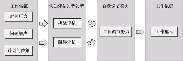
问卷包括4个变量:自变量即工作特征, 包括时间压力、问题解决和计划与决策三个维度; 两个中介变量即认知评估过程和自我调节努力, 其中认知评估过程包括挑战评估和阻碍评估两个维度; 因变量即工作场所拖延; 睡眠质量和职业自我效能感作为控制变量。被试内和被试间两个水平的假设一致, 均如图3所示: 假设1是工作特征通过增加挑战评估来减少自我调节努力从而减少影响工作场所拖延; 假设2是工作特征通过增加阻碍评估来增加自我调节努力从而增加工作场所拖延。
图3
由于数据为嵌套结构, 因此研究者采用多层结构方程模型进行分析, 将变量方差分解至被试间部分和被试内部分。相较于其他多层中介分析, 结构方程建模产生的偏差更小。此外, 大多数情况下被试内水平的间接效应呈现偏态分布, 因此采用贝叶斯估计还可以更好地检验间接效应(Preacher, Zyphur, & Zhang, 2010)。
研究者采用Mplus 8.0进行贝叶斯多层结构方程模型分析, 结果表明模型拟合良好, PPp值为0.460。参数估计结果表明:被试内水平中, 工作特征的三个维度均对工作场所拖延有负向的序列间接效应, 即通过增加挑战评估来减少自我调节努力, 从而影响工作场所拖延(时间压力: 间接效应大小为-0.004, 95% CI [-0.009, -0.000]; 问题解决: 间接效应大小为-0.011, 95% CI [-0.023, -0.002]; 计划与决策: 间接效应大小为-0.004, 95% CI [-0.009, -0.000])。此外, 时间压力对工作场所拖延还有正向的序列间接效应, 即通过增加阻碍评估来增加自我调节努力从而影响工作场所拖延(间接效应大小为0.006, 95% CI [0.002, 0.012])。而在被试间水平中, 上述的序列间接效应并不成立。因此, 该研究揭示了工作特征与工作场所拖延存在密切关系, 且主要通过被试内水平上的认知评估和自我调节努力来实现的。
4 模型评价与拟合指标
传统的模型拟合指标并不适用于贝叶斯估计, 因此在使用贝叶斯方法时, 需要用到以下指标对模型进行有效的评估。
4.1 后验预测p值
模型和数据的拟合程度可以通过后验预测检验来进行评估(Gelman, Meng, Stern, & Rubin, 1996)。后验预测检验比较了实际数据与假设模型产生的数据之间的差异, 可以用于评估模型和实际数据的拟合程度。通过后验预测检验可以得到后验预测p值(Posterior Predictive p-value, PPp值)。PPp值与假设检验中的p值含义不同, 它是指在MCMC算法多次迭代中, 依据理论模型生成的统计检验量大于样本数据的统计检验量的比例。因此, PPp值在0.5左右, 即接近随机概率1/2时, 表示模型拟合得很好。此外, 后验预测检验还能够给出样本数据与模型生成数据之间统计检验量差异的95%置信区间, 当该区间的下限为负数, 且0落在区间中心时, 表示模型拟合得很好(Muthén & Asparouhov, 2012)。
4.2 贝叶斯因子
贝叶斯因子(Bayes Factor)是用于模型比较的重要统计量, 它可用于比较非嵌套模型。它可以比较在已有数据集下, 支持M0与M1两个模型的概率。这样的比较不依赖于假设检验, 即使样本量很大也不会倾向于支持备择假设M1 (李锡钦, 2011)。Kass和Raftery (1995)提出了解释贝叶斯因子的准则。如, 贝叶斯因子介于1到3之间表示该数据对两个模型的支持程度差不多, 此时在模型选择时还需要考虑“简约性”原则, 或结合其他指标进行判断。
4.3 贝叶斯信息准则
贝叶斯信息准则(Bayesian Information Criterion, BIC; Schwarz, 1978)与赤池信息准则(Akaike Information Criterion, AIC)一样, 在评价模型拟合的同时考虑了模型复杂度, 对复杂的模型进行惩罚, 且BIC比起AIC对复杂模型的惩罚作用更强。BIC的值越小, 说明该模型拟合更好。但BIC是相对拟合指标, 不能评价两个模型拟合差异的显著性。
4.4 偏差信息准则
与BIC一样, 偏差信息准则(Deviance Information Criterion, DIC)也被用来比较竞争模型(Spiegelhalter, Best, Carlin, & van der Linde, 2002)。DIC越小表示模型拟合越好。但是由于DIC更加符合贝叶斯偏差(Bayesian Deviance)的概念(Kaplan & Depaoli, 2012), 其应用更为普遍。相比之下, BIC更多被用于频率学方法中的模型比较。
5 软件介绍
尽管采用贝叶斯方法估计SEM有着诸多优点, 但其应用一直较为滞后, 一个重要的原因就是它看起来要求研究者具备很好的贝叶斯统计基础(Muthén & Asparouhov, 2012)。但实际上目前能够采用贝叶斯方法分析SEM的软件不仅可以满足大多数研究者的需求, 而且易于学习使用。其中常用软件主要有以下几个, 除Mplus外其余软件均为免费开源软件:
(1) 目前最为流行的潜变量分析软件Mplus (Muthén & Muthén, 1998~2019),其编程语言简单易学,由于其默认设定较多,在使用中研究者一般只需要将估计方法从极大似然估计换为贝叶斯估计,并提供相应先验信息即可。如果没有提供先验信息Mplus通常会默认提供无信息先验分布。此外, Mplus软件的更新速度很快, Mplus 8.3版本已经可以估计贝叶斯潜调节模型(即调节变量为潜变量的模型)、贝叶斯渐近测量不变性模型等。而当研究者将估计方法设定为贝叶斯估计时, Mplus 8.3可以提供PPp值、DIC和BIC值作为模型拟合与评价的指标;
(2) WinBUGS (Windows version of Bayesian Inference Using Gibbs Sampling; Lunn et al., 2000)是专门用于贝叶斯统计推断的软件包。相比于Mplus, 其对研究者的贝叶斯统计基础有更高的要求。Mplus中一些默认的估计设定在WinBUGS中需要研究者自己设定, 但是它功能强大, 可以灵活地对复杂模型进行估计。WinBUGS能提供DIC值作为模型拟合与评价的指标;
(3) 软件Stan (Stan Development Team, 2014)可以对复杂的BSEM(如潜调节模型、多层模型等)进行估计, 且可以与最流行的数据分析语言(如R, Matlab, Python等)接口;
(4) R软件中的blavaan包(Merkle, & Rosseel, 2015)尚不能估计一些特殊的模型, 如潜调节模型、含有序分类变量的模型等。不过用户可以根据需要导出JAGS (Just Another Gibbs Sampler; Plummer, 2005)代码来估计复杂、特殊的模型。此外, 通过mplus2lavaan()函数还可以将Mplus软件与blavaan接口。blavaan能提供PPp值以及DIC值作为模型拟合与评价的指标。
在本文所介绍的应用研究中, 大部分研究都采用了Mplus软件进行贝叶斯结构方程建模(例如, Crenshaw et al., 2016; Falkenström et al., 2015; Golay et al., 2013; Zeman et al., 2017), 但也有两篇研究采用R和JAGS软件进行建模(Praetorius, Koch, Scheunpflug, Zeinz, & Dresel, 2017; Winans- Mitrik et al., 2014)。研究者可以根据自己的建模需要选择相应的分析软件。
6 讨论
在结构方程建模中贝叶斯方法有着无可替代的优势, 在模型识别和拟合, 参数估计, 处理复杂模型和小样本情况等方面贝叶斯方法都有着更好的表现。该方法在近几年的发展也颇为迅猛(van de Schoot et al., 2017)。基于贝叶斯方法结合先验信息, 不依赖方差协方差矩阵等特性, 衍生出了新的建模思路, 如放宽对传统测量模型的严格限制(Lu et al., 2016; Muthén & Asparouhov, 2012; Pan et al., 2017), 多组模型中允许组间存在较小的差异(Muthén & Asparouhov, 2013)等, 而这些建模思路在传统方法中都难以实现。
但是截至2018年6月, 在中国知网数据库检索发现, 在国内心理学期刊中尚未有贝叶斯结构方程模型的应用研究。希望本文可以为国内心理学研究者在实证研究中提供新的思路, 在应对小样本、传统方法下模型无法识别等情况时可以游刃有余。此外, 频率学派方法的主导地位使得心理学研究者对贝叶斯方法的了解不足。王孟成等人(2017)也指出学术界对贝叶斯的了解是相当有限的, 这使得应用研究者在面对这种新的研究工具时可能会担心无法很好地掌握这种方法。但实际上对于有结构方程建模基础的研究者来说, 采用Mplus软件进行贝叶斯估计是非常易于掌握的, 希望本文的介绍可以打破这种刻板印象。
尽管使用贝叶斯方法有着诸多优势, 但先验的潜在影响、贝叶斯特征与结果的错误解读, 以及不正确的贝叶斯结果报告都可能带来错误。针对以上几点潜在的危险, Depaoli和van de Schoot (2015)提出了WAMBS清单以避免贝叶斯方法的误用, 研究者可以参考这个清单以避免结果报告的错误。而随着采用贝叶斯方法估计结构方程模型的应用和方法研究越来越多(van de Schoot et al., 2017), 相信其建模方法、使用技巧和报告规范会越来越完善。
参考文献
Double dissociation between the neural correlates of the general and specific factors of the life orientation test-revised
Exploratory structural equation modeling
Bayesian analysis of latent variable models using Mplus. (Technical Report)
General random effect latent variable modeling: Random subjects, items, contexts, and parameters
Retrieved from .
Multiple-group factor analysis alignment
Bayesian methods for the analysis of small sample multilevel data with a complex variance structure
DOI:10.1037/a0030642
Magsci
[本文引用: 2]

Inferences from multilevel models can be complicated in small samples or complex data structures. When using (restricted) maximum likelihood methods to estimate multilevel models, standard errors and degrees of freedom often need to be adjusted to ensure that inferences for fixed effects are correct. These adjustments do not address problems in estimating variance/covariance components. An alternative to the adjusted likelihood method is to use Bayesian methods, which can produce accurate inferences about fixed effects and variance/covariance parameters. In this article, the authors contrast the benefits and limitations of likelihood and Bayesian methods in the estimation of multilevel models. The issues are discussed in the context of a partially clustered intervention study, a common intervention design that has been shown to require an adjusted likelihood analysis. The authors report a Monte Carlo study that compares the performance of an adjusted restricted maximum likelihood (REML) analysis to a Bayesian analysis. The results suggest that for fixed effects, the models perform equally well with respect to bias, efficiency, and coverage of interval estimates. Bayesian models with a carefully selected gamma prior for the variance components were more biased but also more efficient with respect to estimation of the variance components than the REML model. However, the results also show that the inferences about the variance components in partially clustered studies are sensitive to the prior distribution when sample sizes are small. Finally, the authors compare the results of a Bayesian and adjusted likelihood model using data from a partially clustered intervention trial.
Latent curve models: A structural equation approach. Hoboken, NJ: Wiley-
Model modification in covariance structure modeling: A comparison among likelihood ratio, Lagrange multiplier, and Wald tests
A nondegenerate penalized likelihood estimator for variance parameters in multilevel models
DOI:10.1007/s11336-013-9328-2
Magsci
[本文引用: 1]
Group-level variance estimates of zero often arise when fitting multilevel or hierarchical linear models, especially when the number of groups is small. For situations where zero variances are implausible a priori, we propose a maximum penalized likelihood approach to avoid such boundary estimates. This approach is equivalent to estimating variance parameters by their posterior mode, given a weakly informative prior distribution. By choosing the penalty from the log-gamma family with shape parameter greater than 1, we ensure that the estimated variance will be positive. We suggest a default log-gamma(2,lambda) penalty with lambda -> 0, which ensures that the maximum penalized likelihood estimate is approximately one standard error from zero when the maximum likelihood estimate is zero, thus remaining consistent with the data while being nondegenerate. We also show that the maximum penalized likelihood estimator with this default penalty is a good approximation to the posterior median obtained under a noninformative prior.<br/>Our default method provides better estimates of model parameters and standard errors than the maximum likelihood or the restricted maximum likelihood estimators. The log-gamma family can also be used to convey substantive prior information. In either case-pure penalization or prior information-our recommended procedure gives nondegenerate estimates and in the limit coincides with maximum likelihood as the number of groups increases.
Revised scoring and improved reliability for the communication patterns questionnaire
Psychometric evaluation of the overexcitability questionnaire-two applying Bayesian structural equation modeling (BSEM) and multiple-group BSEM-based alignment with approximate measurement invariance
A Bayesian approach to multilevel structural equation modeling with continuous and dichotomous outcomes
Improving transparency and replication in Bayesian statistics: The wambs-checklist
Assessment and propagation of model uncertainty
Confirmatory factor analysis of the patient version of the working alliance inventory-short form revised
Testing gender invariance of the hospital anxiety and depression scale using the classical approach and Bayesian approach
DOI:10.1007/s11136-013-0594-3
Magsci
[本文引用: 2]
Measurement invariance is an important attribute for the Hospital Anxiety and Depression Scale (HADS). Most of the confirmatory factor analysis studies on the HADS adopt the classical maximum likelihood approach. The restrictive assumptions of exact-zero cross-loadings and residual correlations in the classical approach can lead to inadequate model fit and biased parameter estimates. The present study adopted both the classical approach and the alternative Bayesian approach to examine the measurement and structural invariance of the HADS across gender.<br/>A Chinese sample of 326 males and 427 females was used to examine the two-factor model of the HADS across gender. Configural and scalar invariance of the HADS were evaluated using the classical approach with the robust-weighted least-square estimator and the Bayesian approach with zero-mean, small-variance informative priors to cross-loadings and residual correlations.<br/>Acceptable and excellent model fits were found for the two-factor model under the classical and Bayesian approaches, respectively. The two-factor model displayed scalar invariance across gender using both approaches. In terms of structural invariance, females showed a significantly higher mean in the anxiety factor than males under both approaches.<br/>The HADS demonstrated measurement invariance across gender and appears to be a well-developed instrument for assessment of anxiety and depression. The Bayesian approach is an alternative and flexible tool that could be used in future invariance studies.
Bayesian data analysis (3rd ed
.).
Bayesian data analysis
.
Posterior predictive assessment of model fitness via realized discrepancies
Further insights on the French WISC-IV factor structure through Bayesian structural equation modeling
DOI:10.1037/a0030676
Magsci
[本文引用: 2]
The interpretation of the Wechsler Intelligence Scale for Children-Fourth Edition (WISC-IV) is based on a 4-factor model, which is only partially compatible with the mainstream Cattell-Horn-Carroll (CHC) model of intelligence measurement. The structure of cognitive batteries is frequently analyzed via exploratory factor analysis and/or confirmatory factor analysis. With classical confirmatory factor analysis, almost all cross-loadings between latent variables and measures are fixed to zero in order to allow the model to be identified. However, inappropriate zero cross-loadings can contribute to poor model fit, distorted factors, and biased factor correlations; most important, they do not necessarily faithfully reflect theory. To deal with these methodological and theoretical limitations, we used a new statistical approach, Bayesian structural equation modeling (BSEM), among a sample of 249 French-speaking Swiss children (8-12 years). With BSEM, zero-fixed cross-loadings between latent variables and measures are replaced by approximate zeros, based on informative, small-variance priors. Results indicated that a direct hierarchical CHC-based model with 5 factors plus a general intelligence factor better represented the structure of the WISC-IV than did the 4-factor structure and the higher order models. Because a direct hierarchical CHC model was more adequate, it was concluded that the general factor should be considered as a breadth rather than a superordinate factor. Because it was possible for us to estimate the influence of each of the latent variables on the 15 subtest scores, BSEM allowed improvement of the understanding of the structure of intelligence tests and the clinical interpretation of the subtest scores.
Sensitivity analysis, Monte Carlo risk analysis, and Bayesian uncertainty assessment
The effect of estimation method and sample size in multilevel structural equation modeling
Forced zero cross-loading misspecifications in measurement component of structural equation models: Beware of even “small” misspecifications
Perceived emotional social support in bereaved spouses mediates the relationship between anxiety and depression
Social influence interpretation of interpersonal processes and team performance over time using Bayesian model selection
Structural equation modeling: Foundations and extensions (2nd ed.).
Bayesian structural equation modeling. In R. H. Hoyle (Ed.), Handbook of structural equation modeling (pp. 650-673)
Bayes factors
Lower level mediation in multilevel models
Measurement invariance testing with many groups: A comparison of five approaches
Basic and advanced Bayesian structural equation modeling
Sample size limits for estimating upper level mediation models using multilevel SEM
Bayesian factor analysis as a variable-selection problem: Alternative priors and consequences
WinBUGS-a Bayesian modelling framework: Concepts, structure, and extensibility
DOI:10.1023/A:1008929526011
Magsci
<a name="Abs1"></a>WinBUGS is a fully extensible modular framework for constructing and analysing Bayesian full probability models. Models may be specified either textually via the BUGS language or pictorially using a graphical interface called DoodleBUGS. WinBUGS processes the model specification and constructs an object-oriented representation of the model. The software offers a user-interface, based on dialogue boxes and menu commands, through which the model may then be analysed using Markov chain Monte Carlo techniques. In this paper we discuss how and why various modern computing concepts, such as object-orientation and run-time linking, feature in the software's design. We also discuss how the framework may be extended. It is possible to write specific applications that form an apparently seamless interface with WinBUGS for users with specialized requirements. It is also possible to interface with WinBUGS at a lower level by incorporating new object types that may be used by WinBUGS without knowledge of the modules in which they are implemented. Neither of these types of extension require access to, or even recompilation of, the WinBUGS source-code.
Model modifications in covariance structure analysis: The problem of capitalization on chance
Confidence limits for the indirect effect: Distribution of the product and resampling methods
Cross-language associations in the development of preschoolers’ receptive and expressive vocabulary
Exploratory structural equation modeling, integrating CFA and EFA: Application to students’ evaluations of university teaching
A Monte Carlo sample size study: How many countries are needed for accurate multilevel SEM?
Power in Bayesian mediation analysis for small sample research
Bayesian structural equation modeling: A more flexible representation of substantive theory
BSEM measurement invariance analysis
Mplus user’s guide. Eighth Edition. Los Angeles, CA: Muthén &
A default Bayesian hypothesis test for mediation
An alternative to post hoc model modification in confirmatory factor analysis: The Bayesian lasso
JAGS: Just Another Gibbs Sampler.
Identifying determinants of teachers' judgment (in) accuracy regarding students' school-related motivations using a Bayesian cross-classified multi-level model
Alternative methods for assessing mediation in multilevel data: The advantages of multilevel SEM
A general multilevel SEM framework for assessing multilevel mediation
Procrastination in daily working life: A diary study on within-person processes that link work characteristics to workplace procrastination
Generalized multilevel structural equation modeling
DOI:10.1007/BF02295939
Magsci
[本文引用: 1]
<a name="Abs1"></a>A unifying framework for generalized multilevel structural equation modeling is introduced. The models in the framework, called generalized linear latent and mixed models (GLLAMM), combine features of generalized linear mixed models (GLMM) and structural equation models (SEM) and consist of a response model and a structural model for the latent variables. The response model generalizes GLMMs to incorporate factor structures in addition to random intercepts and coefficients. As in GLMMs, the data can have an arbitrary number of levels and can be highly unbalanced with different numbers of lower-level units in the higher-level units and missing data. A wide range of response processes can be modeled including ordered and unordered categorical responses, counts, and responses of mixed types. The structural model is similar to the structural part of a SEM except that it may include latent and observed variables varying at different levels. For example, unit-level latent variables (factors or random coefficients) can be regressed on cluster-level latent variables. Special cases of this framework are explored and data from the British Social Attitudes Survey are used for illustration. Maximum likelihood estimation and empirical Bayes latent score prediction within the GLLAMM framework can be performed using adaptive quadrature in gllamm, a freely available program running in Stata.
Testing students' e-learning via facebook through Bayesian structural equation modeling
Becoming more specific: Measuring and modeling teachers' perceived usefulness of ICT in the context of teaching and learning
Measurement invariance: Review of practice and implications
DOI:10.1016/j.hrmr.2008.03.003
Magsci
[本文引用: 2]
<h2 class="secHeading" id="section_abstract">Abstract</h2><p id="">A review of efforts to assess the invariance of measurement instruments across different respondent groups using confirmatory factor analysis (CFA) is provided for the years since the Vandenberg and Lance [Vandenberg, R. J., & Lance, C. E. (2000). A review and synthesis of the measurement invariance literature: Suggestions, practices, and recommendations for organizational research. Organizational Research Methods, 3, 4–69.] review. Investigators are more frequently reporting tests of scalar invariance and tests for differences in latent factor means and partial invariance. Efforts have been made to assess, the impact of the choice of a referent indicator in multi-group studies, the appropriateness of forming partials as indicators of a latent construct, the degree of convergence of item response theory and CFA analyses of measurement differences across groups, and the implications of findings of invariance. In this context, a demonstration of the impact of partial invariance on estimated group differences in reliability and means is provided and discussed.</p>
Estimating the dimension of a model
Psychological needs, engagement, and work intentions: A Bayesian multi-measurement mediation approach and implications for HRD. European
Model modification
Bayesian measures of model complexity and fit (with discussion)
Stan modeling language: Users guide and reference manual, Version 2.2.0.
Interpersonal emotion regulation among adolescent athletes: A Bayesian multilevel model predicting sport enjoyment and commitment
.
R mediation: An R package for mediation analysis confidence intervals
DOI:10.3758/s13428-011-0076-x
Magsci
[本文引用: 1]
This article describes the RMediation package, which offers various methods for building confidence intervals (CIs) for mediated effects. The mediated effect is the product of two regression coefficients. The distribution-of-the-product method has the best statistical performance of existing methods for building CIs for the mediated effect. RMediation produces CIs using methods based on the distribution of product, Monte Carlo simulations, and an asymptotic normal distribution. Furthermore, RMediation generates percentiles, quantiles, and the plot of the distribution and CI for the mediated effect. An existing program, called PRODCLIN, published in Behavior Research Methods, has been widely cited and used by researchers to build accurate CIs. PRODCLIN has several limitations: The program is somewhat cumbersome to access and yields no result for several cases. RMediation described herein is based on the widely available R software, includes several capabilities not available in PRODCLIN, and provides accurate results that PRODCLIN could not.
Monte Carlo confidence intervals for complex functions of indirect effects
A systematic review of Bayesian articles in psychology: The last 25 years
A review and synthesis of the measurement invariance literature: Suggestions, practices, and recommendations for organizational research
Moderated mediation analysis using Bayesian methods
Description of an intensive residential aphasia treatment program: Rationale, clinical processes, and outcomes
DOI:10.1044/2014_AJSLP-13-0102
Magsci
[本文引用: 1]
Purpose: The purpose of this article is to describe the rationale, clinical processes, and outcomes of an intensive comprehensive aphasia program (ICAP).<br/>Method: Seventy-three community-dwelling adults with aphasia completed a residentially based ICAP. Participants received 5 hr of daily 1:1 evidence-based cognitivelinguistically oriented aphasia therapy, supplemented with weekly socially oriented and therapeutic group activities over a 23-day treatment course. Standardized measures of aphasia severity and communicative functioning were obtained at baseline, program entry, program exit, and follow-up.<br/>Results were analyzed using a Bayesian latent growth curve model with 2 factors representing (a) the initial level and (b) change over time, respectively, for each outcome measure. Results: Model parameter estimates showed reliable improvement on all outcome measures between the initial and final assessments. Improvement during the treatment interval was greater than change observed across the baseline interval, and gains were maintained at follow-up on all measures.<br/>Conclusions: The rationale, clinical processes, and outcomes of a residentially based ICAP have been described. ICAPs differ with respect to treatments delivered, dosing parameters, and outcomes measured. Specifying the defining components of complex interventions, establishing their feasibility, and describing their outcomes are necessary to guide the development of controlled clinical trials.
Bayesian mediation analysis
Maternal incarceration, children’s psychological adjustment, and the mediating role of emotion regulation
Bayesian analysis of longitudinal data using growth curve models
